What the Loss Curve Doesn't Tell You

A note on the charts: they come straight out of my experiment records, so their titles carry labels like “Experiment 027” that only mean something in my notes. The axes and curves are what matter.

My last post was about training decisions like schedules, optimizers, dropout, and batch size. This one looks at training as a system, the process that runs the model. Where the time goes, whether a run can be stopped and restarted without changing what it learns, what happens when the numbers go bad, where the memory goes, and how many CPU threads I should have been using all along.

None of the five experiments here changes a line of the model or the training math. Each one adds an instrument to the loop and reads what comes back.

In four of the five, something had been wrong for a while and was invisible in the one number I was watching. A mishandled restart keeps producing a falling loss. A memory estimate can be off by a factor of 27 while every run completes. A thread count can be wrong for four experiments in a row without a symptom. The loss curve measures the model, and almost everything in this post is a property of the process running it.

Memory and Profiler Instrumentation

The training script already logged step time, tokens per second, gradient norm, and loss. The one gap was memory: nothing recorded how much RAM the process used, or whether that stayed put over a forty-minute run. The fix is one line:

def peak_memory_mb() -> float:
    return resource.getrusage(resource.RUSAGE_SELF).ru_maxrss / 1024

ru_maxrss is peak resident set size, the most physical memory the process has had in use since it started. The operating system tracks it whether anyone reads it or not, and I had simply never read it.

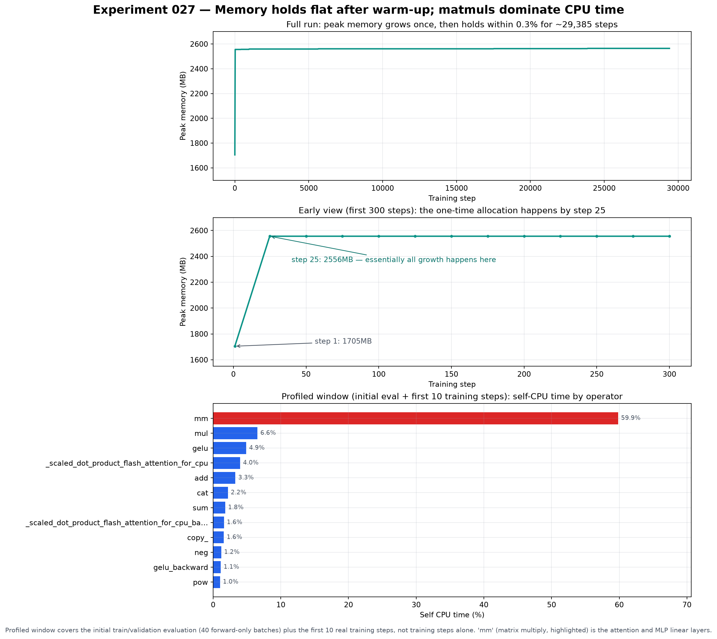
The chart shows peak memory over the full run, a zoom on the first few steps, and the profiler’s breakdown of time by operation. The memory curve is exactly what “no leak” should look like. Almost all the growth, from 1,704.8MB to 2,555.7MB, happens by step 25, the one-time allocation of parameters, gradients, and the optimizer’s two running-average buffers. The remaining 29,385 steps add 8.6MB. I’d assumed a fixed model at a fixed batch size couldn’t leak, but watching the number hold flat for forty minutes is different from assuming it.

The second instrument was PyTorch’s profiler, which shows where the CPU spends its time in a forward and backward pass. It reports self time (time in an operation’s own code) and total time (including operations it calls into). I read self time throughout, because it credits time to the operation that actually spent the cycles.

Matrix multiplies dominating was expected, since attention projections and linear layers are nearly the whole model. But their share moved a lot between two runs: 81% in a short smoke test and 59.85% in the real one. The main difference was the thread count, 4 against 20. I left that as a loose end, and it became the last section of this post.

One thing this didn’t answer: the Mixture of Experts post ended by asking how much of that model’s runtime was real expert work versus the masking and gathering around it. This pass profiled the dense baseline, so that’s still open.

The number I couldn’t explain was the peak itself. Peak memory was around 2.56GB, but parameters, gradients, and optimizer state for a 5,837,056-parameter model account for about 93MB. That factor of 27 is why the memory experiment further down exists.

What a Checkpoint Has to Contain

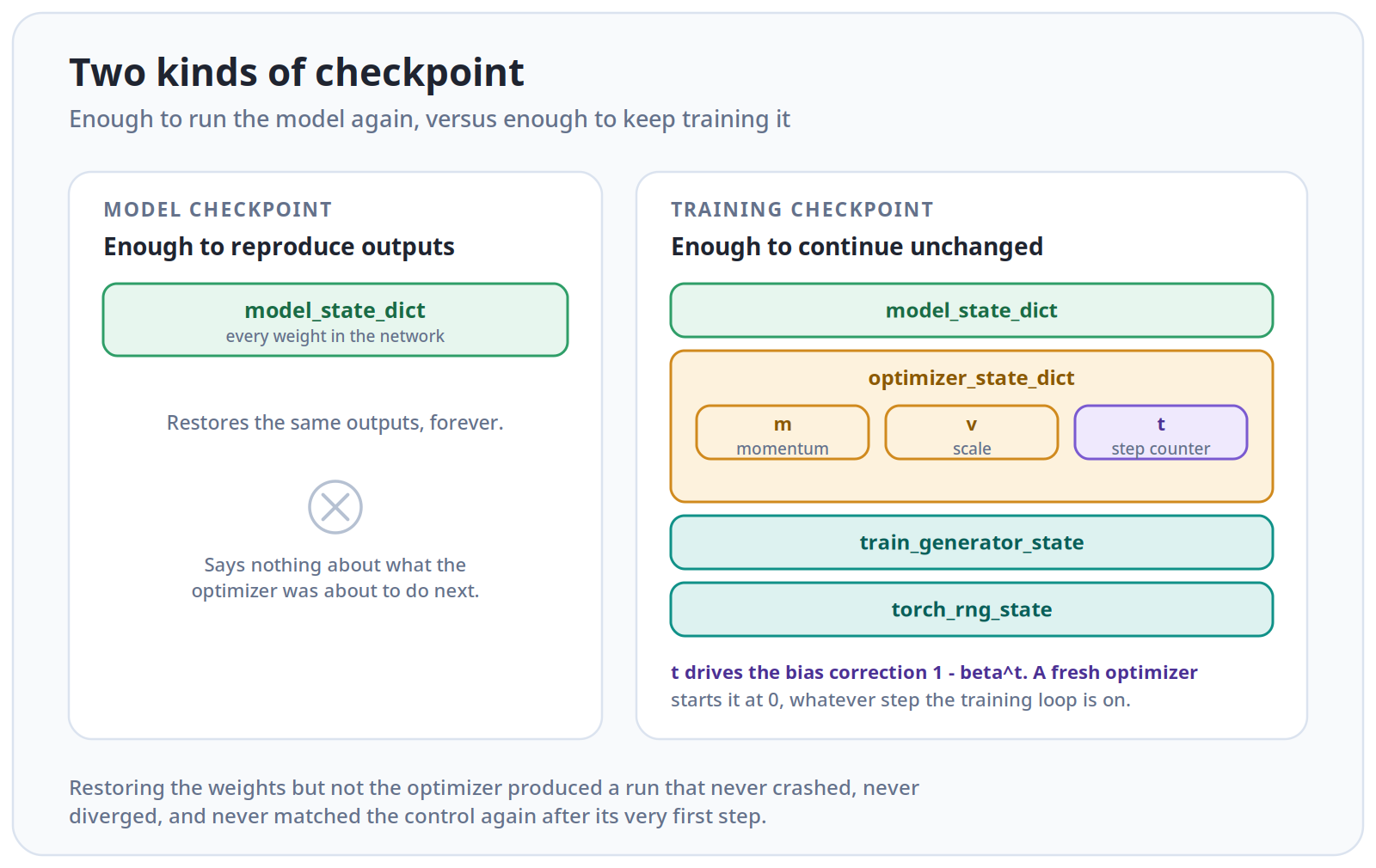
Weights alone reproduce the model’s output exactly. They aren’t enough to keep training it identically, because the optimizer carries state the next update depends on. AdamW keeps two running averages per parameter: m, the momentum term, and v, a sense of how large and noisy gradients have been. It also keeps its own step counter, t.

That counter is the key part. m and v start at zero, so AdamW corrects the early bias by dividing by 1 - beta^t, which is a large correction early and almost nothing later. A fresh optimizer starts at t = 0 with empty m and v, whatever step the training loop thinks it’s on. Give it the right weights and the right next batch and it will still compute a different update, because it thinks it’s at the beginning.

So the checkpoint has to hold more than weights:

checkpoint = {
    "step": step,
    "model_state_dict": model.state_dict(),
    "optimizer_state_dict": optimizer.state_dict(),
    "train_generator_state": train_generator.get_state(),
    "torch_rng_state": torch.get_rng_state(),
    "training_metrics": training_metrics,
    "evaluation_metrics": evaluation_metrics,
    "training_time": training_time,
}

Each field answers something the next process needs to know: which weights, what the optimizer was about to do, which batch comes next (batch sampling has its own generator), what random operations like dropout will draw next, and what to report for the full run.

I ran four arms: a control running 4,000 steps straight through, an identical run that checkpoints at step 2,000, a resume that restores everything from that checkpoint, and a deliberately wrong resume that restores everything except the optimizer state.

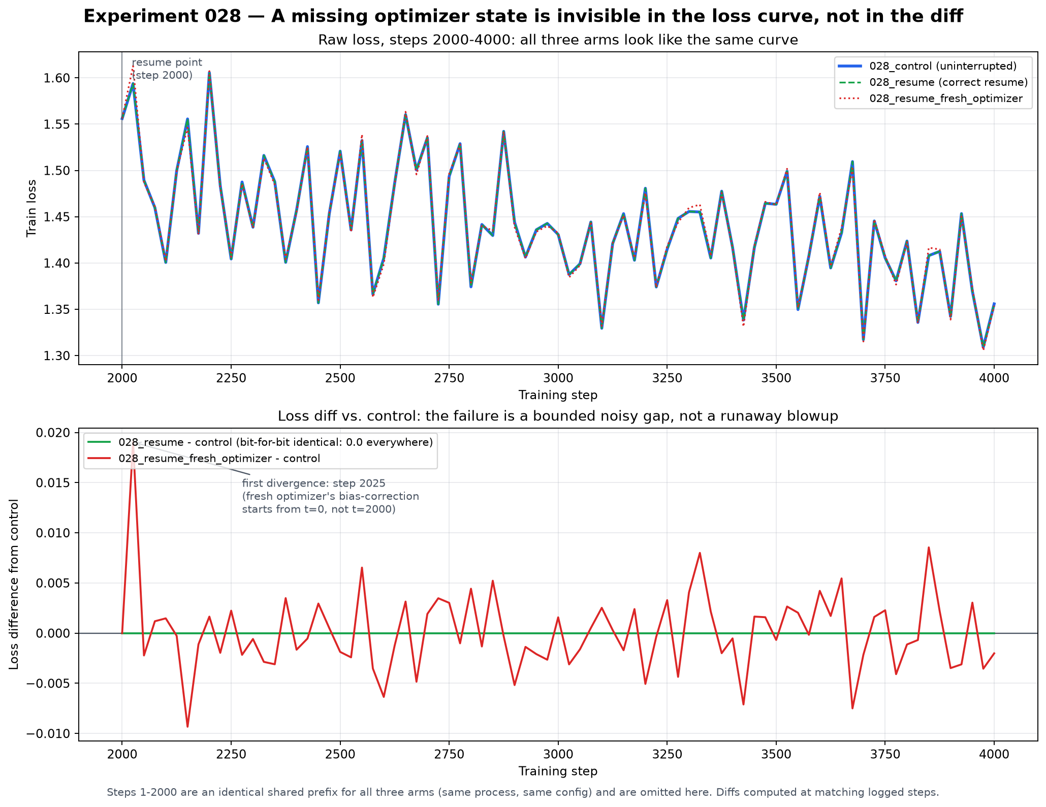
The top panel shows loss for each arm, and the bottom shows each arm’s difference from the control. The correct resume matched the control exactly, at all 161 logged training steps and 17 evaluations after step 2,000, and the generated text was byte-for-byte the same.

The fresh-optimizer arm diverged at the very first logged step after the resume, with a 0.019 gap at step 2,025, the largest single-step difference in the comparison. No ramp into it: the first update already used the wrong m, v, and t. I confirmed the mechanism directly: the saved optimizer’s step field is 2,000, and a fresh one’s is 0.

What I got wrong was the shape. I expected a large divergence, like the optimizer instability in the last post. Instead it was a persistent but bounded gap of roughly 0.0005 to 0.02 that never ran away. A fresh Adam isn’t broken, just less warmed up.

That’s the harder version to catch. The loss goes down, nothing crashes, and the run looks healthy. I’d need a control run beside it to notice, and a real training run doesn’t have one.

Detecting Non-Finite Failures

A training run can fail in two ways. The coupled weight decay run in the last post was slow: it climbed, peaked, and settled onto a worse plateau without ever producing a non-finite number. The other kind is a cliff, where the loss or a gradient overflows float32 and becomes inf or nan, sometimes within two or three steps. By the time a printed loss shows it, the bad update is already in the weights. So the check has to run every step, between the backward pass and the optimizer step:

if not (math.isfinite(loss_value) and math.isfinite(grad_norm)):
    break  # never call optimizer.step() on this

Alongside it I added a periodic safety checkpoint, overwritten in place, so there’s always a recent state to go back to.

Finding a trigger took a search. A learning rate of 8.0 stayed finite for 500-plus steps, with a chaotic loss but no overflow. Every value from 8.05 to 10.0 overflowed by step 3, every time. That’s a sharp edge, so I picked 9.0 and expected a fast failure.

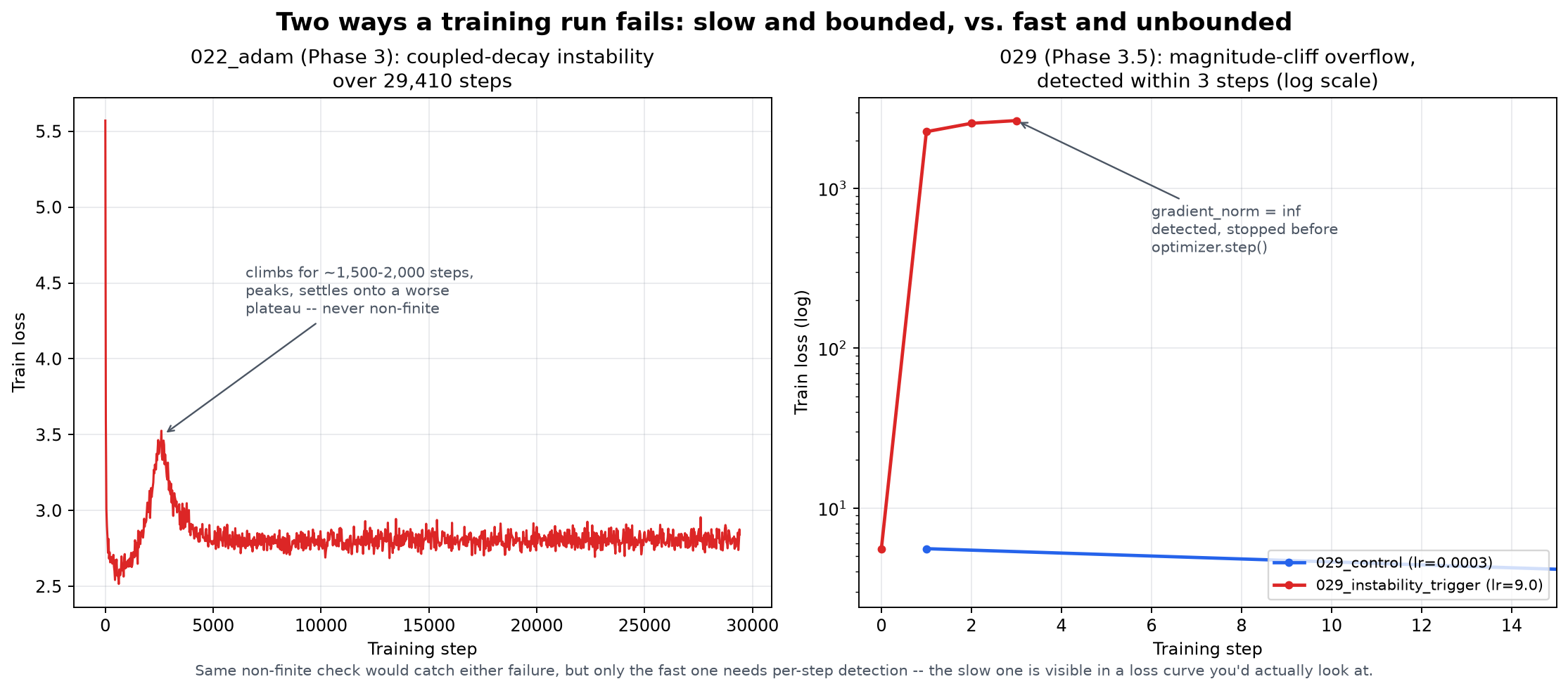
The chart puts the slow failure from the last post next to this one’s overflow, on a log scale. The detector worked: the control ran 2,000 steps with no false positives, and the unstable run was caught at step 3, with a readable diagnostic and a checkpoint on disk.

Then the part I hadn’t planned. I resumed that checkpoint at a safe learning rate, and it failed again immediately, with a loss identical to the original failure down to the last digit: 2659.863525390625. By the time anything looked wrong, the weights had already absorbed two catastrophic updates, and those alone doomed the next forward pass whatever learning rate came after.

“Keep the last checkpoint from before things went wrong” assumes the failure was gradual. Here the last known-good checkpoint was already two bad updates deep. Detecting non-finite values is easy; knowing how far back to rewind is the harder question.

Gradient clipping, the standard fix for instability, made no difference: the clipped run still failed at step 3. clip_grad_norm_ scales by max_norm / total_norm, and with total_norm infinite that scale is 0, and 0 times infinity is NaN. Clipping turns an overflowing gradient from inf into nan. An overflowed gradient has no finite magnitude left to bound.

The Memory Breakdown

This experiment explains the factor of 27, and it starts by splitting memory into three parts that behave very differently:

• Parameters, gradients, and optimizer state are fixed once the model and optimizer exist, and can be computed from the parameter count.
• Process overhead (the interpreter, framework, allocator, and thread pools) is fixed once import torch runs.
• Activation memory is what the forward pass keeps around for the backward pass. It’s the only part that depends on the data shape, and the standard estimate ignores it.

To see where each gets claimed, I read ru_maxrss at nine named points from process start through the first optimizer step. Since it only grows, reading them in order shows where the growth happens.

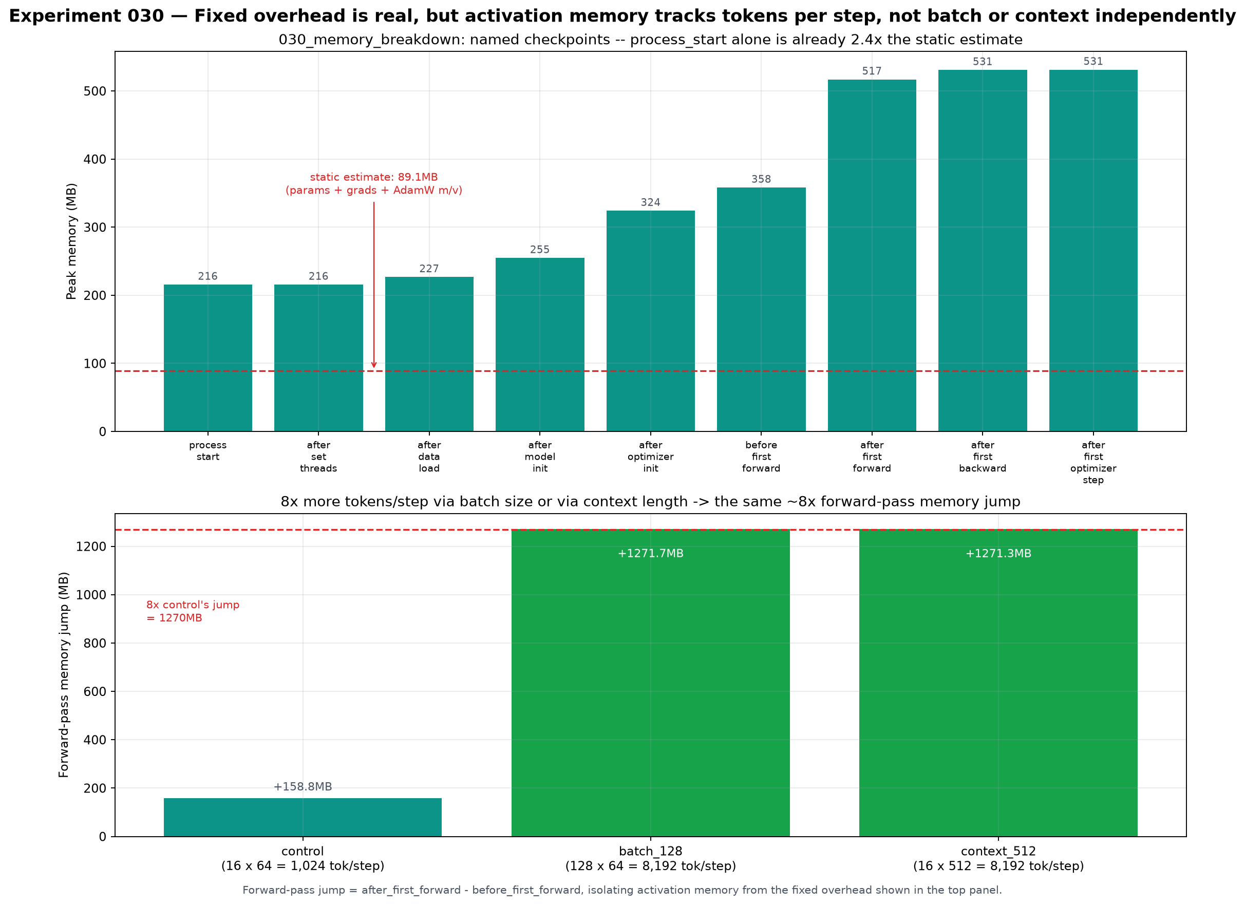
The chart shows the memory at each named point for the control run, plus the batch size and context length sweeps. The fixed overhead was larger than I’d have guessed. At process_start, before the model, data, or optimizer existed, the process was already at 215.67MB, 2.42 times the entire 89.07MB estimate for parameters, gradients, and optimizer state. By the time the optimizer was constructed, it was at 324.11MB. Those numbers were within a third of a megabyte across every arm.

I got the activation result wrong in my prediction. I expected context length to scale worse than batch size, since the attention score matrix is quadratic in context length. It didn’t. An eight-fold batch increase grew forward-pass memory by 8.008 times the control’s. An eight-fold context increase grew it by 8.006 times.

Both sweeps multiply tokens per step by eight, and that’s what memory tracked. Either the CPU kernel never materializes the full attention score tensor, or it’s too small at this model size to register. Either way, quadratic compute and quadratic memory are separate claims, and it’s worth measuring which one actually applies.

One loose end I can’t close. This experiment’s control peaked at 681.98MB, against the observability run’s 2,564MB at the same settings. The earlier run did 29,410 steps instead of 500 and had the profiler attached. Either could plausibly explain the gap, through profiler overhead or allocator fragmentation, and I don’t have the data to say how it splits.

Choosing the Thread Count

Back to the loose end from the first section. Every experiment so far had used 20 threads, a number nobody had chosen deliberately or measured.

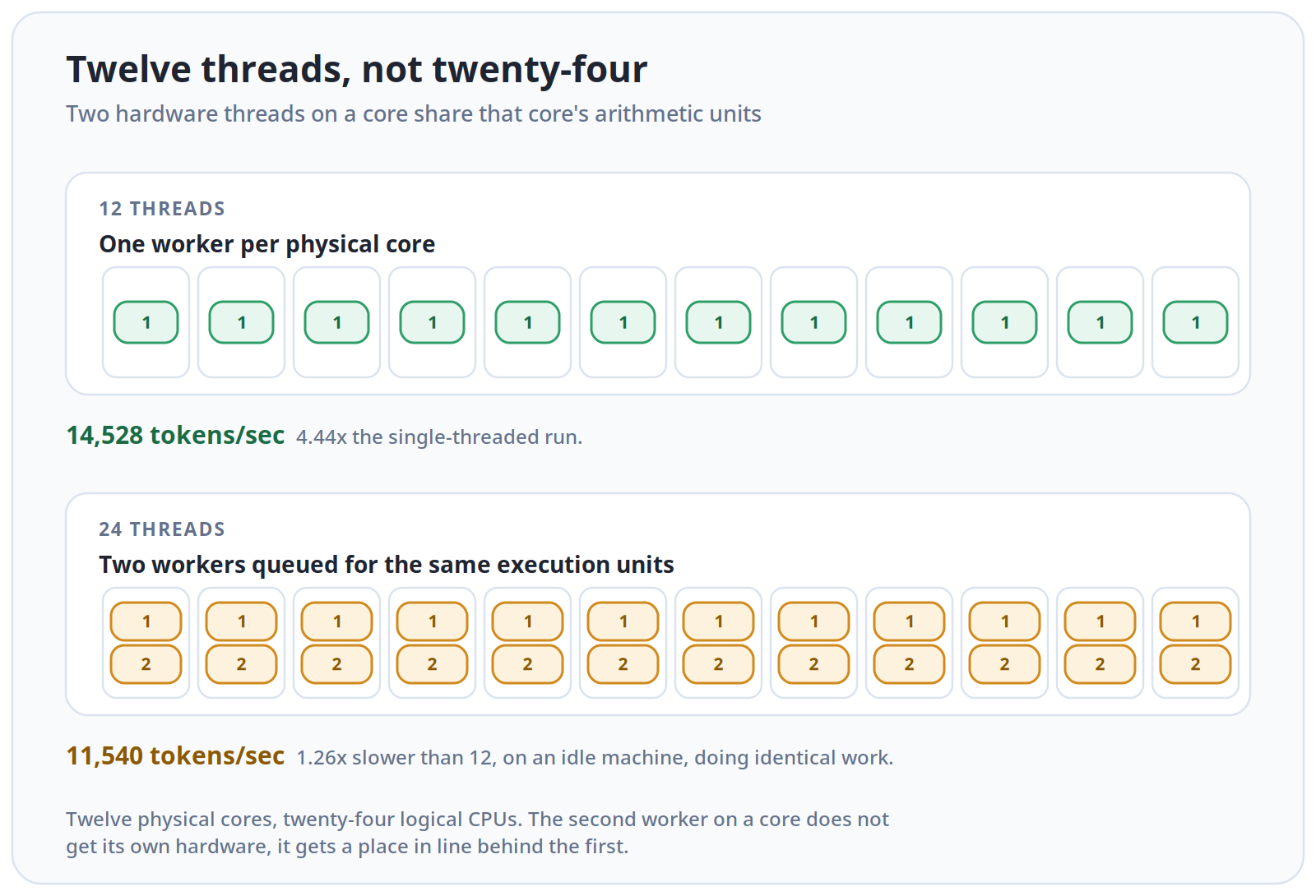
torch.set_num_threads controls how many threads a single operation like a matrix multiply splits its work across. This machine has 12 physical cores, each split into 2 hardware threads, for 24 logical CPUs. The two threads on a core share its arithmetic units rather than doubling them. So 12 threads should give each thread its own core, while 24 should make pairs compete for the same hardware.

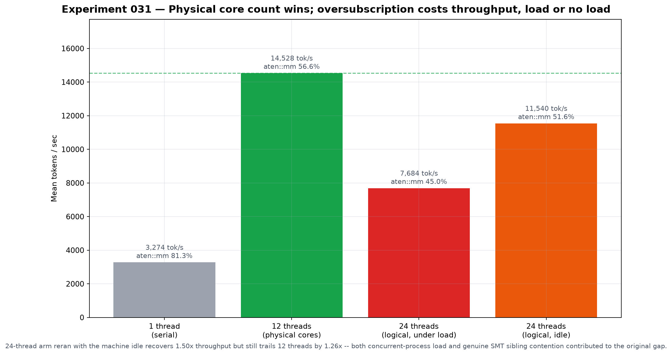
The chart shows throughput at each thread count, plus an idle rerun I’ll get to below. The raw numbers:

 1 thread     3,274.22 tokens/sec    1.00x
12 threads   14,528.50 tokens/sec    4.44x
24 threads    7,684.50 tokens/sec    2.35x

Twelve wins easily, and throughput falls past it. With 24 threads, the same matrix multiplies took nearly twice as long, from 0.862s to 1.564s of self time.

There was a confound worth keeping in. I had other things running on the machine during those runs, which hits the 24-thread arm hardest because it claims every logical CPU. So I reran it with the machine idle.

Both explanations were partly right. Going idle brought 24 threads from 7,684.50 up to 11,540.09 tokens per second, so the competing processes really were a factor. But it was still 1.259 times slower than 12 threads, with matrix multiply self time still higher at 1.003s against 0.862s. That residual is the cost of two threads sharing a core. A confounded result was worth rerunning cleanly rather than trusting it or throwing it out.

One trap in reading the profiler here. The matrix multiply’s share of time fell as threads went up, from 81.33% to 56.62% to 44.96%. But a falling share isn’t the same as getting faster. At 24 threads it’s a smaller slice of a slower run, because thread management overhead grew.

The practical upshot is a one-line change to --threads 12, worth about 4.44 times serial throughput. The method generalizes (measure a few thread counts spanning the physical and logical core counts), but the number 12 is specific to this machine.

Where I Ended Up

I now know what a training checkpoint has to contain and why the optimizer’s step counter is the key part, why clipping can’t save an overflowed gradient, that the framework uses more memory than my model does, that activation memory here tracks tokens per step, and that the right thread count is the physical core count.

The pattern underneath is different from the last post’s. There, changing one setting quietly changed another. Here, the signal I was watching had nothing to say about what was wrong. A resume with a fresh optimizer produced a healthy-looking loss curve on a different trajectory. A memory estimate off by 27 times produced no symptom. A thread count that halved throughput just made runs slower, for four experiments in a row. The loop was reporting on the model, and the fault was somewhere else.

What made them findable was cheap instrumentation pointed at something other than the loss: one line reading a counter the OS already kept, a control run to compare against, a short profiler pass, three runs at different thread counts. None of it required understanding the problem in advance, which was lucky, because in four cases out of five I didn’t.

Next I want to read code I didn’t write. I’ve built this thing twice and instrumented it enough to know how it behaves. The obvious next step is to open a real training codebase and see how much of what I did resembles how it’s actually done.