A note on the charts: they come straight out of my experiment records, so their titles carry labels like “Experiment 020” and “Phase 3” that only mean something in my notes. The axes and curves are what matter.
My last post ended with a list of things I wanted to try that had nothing to do with architecture: learning rate schedules, Adam vs AdamW, dropout, batch size, and reduced precision. The model would stay exactly where it was, and only the training would change.
I expected this to be the tidy part. Every one of those decisions has a standard recommendation, and I mostly wanted to watch them come true on a model small enough to test in an afternoon.
Six of the seven things I ran didn’t come out the way I expected, and they were all wrong in the same way. I’d change one setting, get a result, and later find that it had quietly dragged a second setting along with it. Two results reversed completely once I pinned that second thing down. So this post is less about what learning rate schedules do than about how hard it is to change exactly one thing.
Getting the Baseline to Overfit
Half the decisions on my list are regularizers, and a regularizer has nothing to show on a model that’s still underfitting. So I needed a baseline that overfits.
Two numbers carry the rest of this post. Training loss is how well the model predicts the text it trains on. Validation loss is the same measurement on text held back from training. Overfitting is when the first keeps improving while the second gets worse: the model is learning the specific text rather than the language. The distance between them is the generalization gap. A regularizer is anything that makes memorizing harder, and dropout and weight decay are the two in this post.
My first attempt, a 1.7 million parameter model on 8 MiB of TinyStories, showed no gap at all. So I made the model bigger: 5.8 million parameters, 10 MiB, three passes over the data. Validation loss finished below training loss.
What finally worked was making the dataset smaller. Switching to Tiny Shakespeare, about one megabyte, meant the same forty minutes of compute bought thirty passes instead of three. The overfitting curve showed up on the first try.
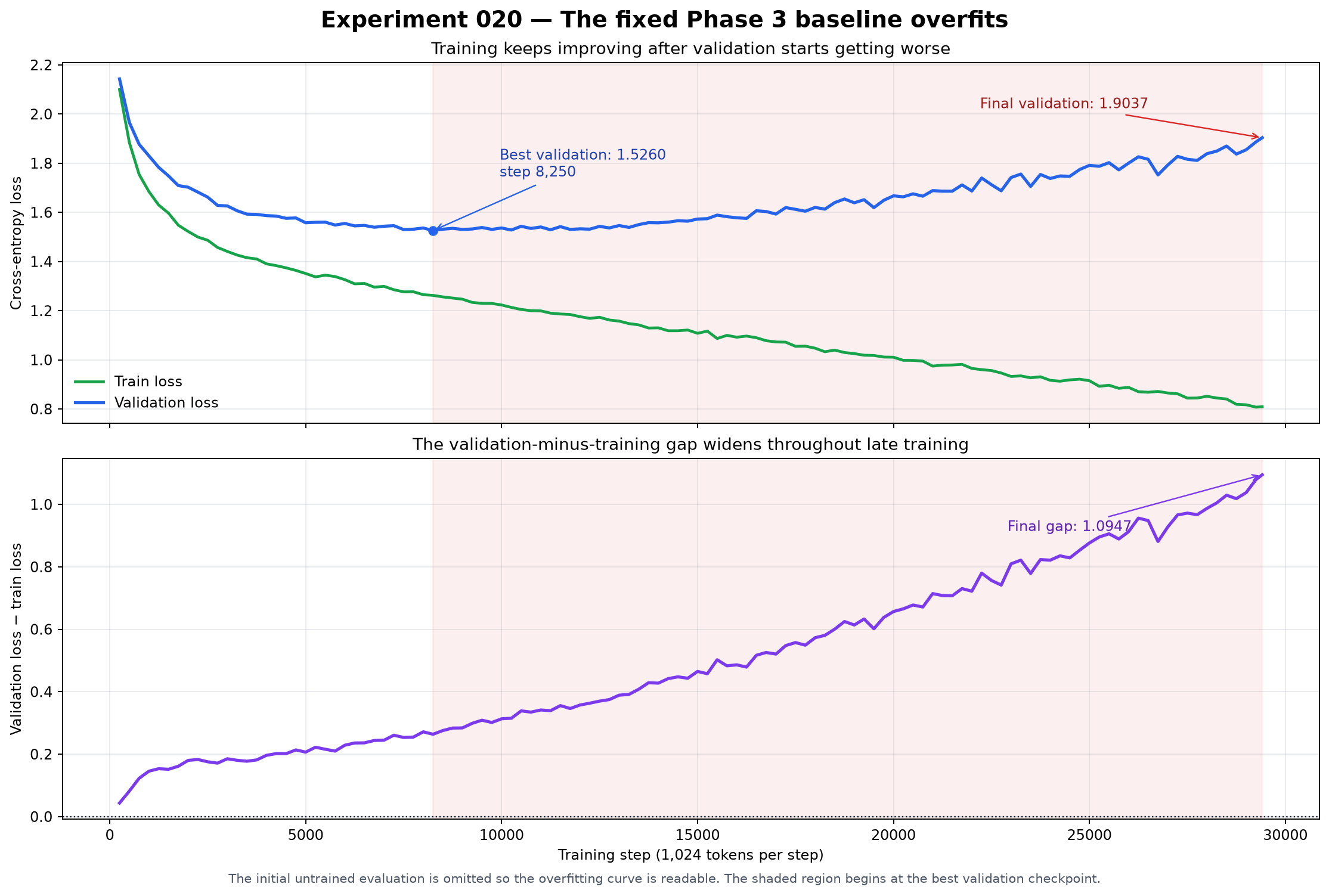
The chart shows training and validation loss over the run. Validation loss bottomed out at 1.5260 around step 8,250, then rose to 1.9037 by the end while training loss kept dropping from 1.2622 to 0.8090. That’s a 25% degradation, and the checkpoint saved at the end is the worst one.
TinyStories is designed to be easy for small models to generalize on, so a held-out story is nearly as predictable as a memorized one. Shakespeare’s dialogue and proper nouns are much richer, so repeated exposure eventually pushed the model from learning the style to learning specific byte sequences. What surprised me was the ordering: two increases in model size did nothing, and one change of dataset did it immediately. Next time a model won’t overfit, I’ll look at the dataset before the parameter count.
The generated text also still looked fine at the end, with correct speaker tags and plausible archaic phrasing. Overfitting was obvious in the loss for half the run and never showed up in the samples at all.
Learning Rate Schedules and Weight Decay
Some vocabulary first. The optimizer takes each step’s gradients and decides how to change each weight. The learning rate is how far it moves them, and a schedule changes that distance over training. Cosine decay eases the rate from full down toward zero along a cosine curve. Warmup ramps it up from zero over the first few hundred steps. Every run in this post got exactly 29,410 steps, so nothing wins by training longer.
The first real experiment was a cosine schedule. My baseline overfits in the back half of training, and cosine takes smaller steps toward the end, so it should do less damage exactly where the damage was happening.
It overfit worse. Final validation loss went from 1.9037 to 2.1337, and adding warmup changed essentially nothing.
What I’d missed is how AdamW applies weight decay. Weight decay is a
small pull toward zero on every weight at every step, and its strength
isn’t the weight_decay setting alone. It’s
learning_rate * weight_decay. At my baseline’s constant
3e-4 and 0.1, that’s a steady
3e-5 shrink per step. Cosine takes the learning rate from
3e-4 down to 3e-5, so by the end the actual
pull is 3e-6. The regularization had decayed to a tenth of
its strength over the course of the run, and the back half is where the
overfitting happens.
So I ran a third arm that scales weight_decay up as the
learning rate comes down, holding the product at 3e-5. If
both effects mattered, it should land in the middle.
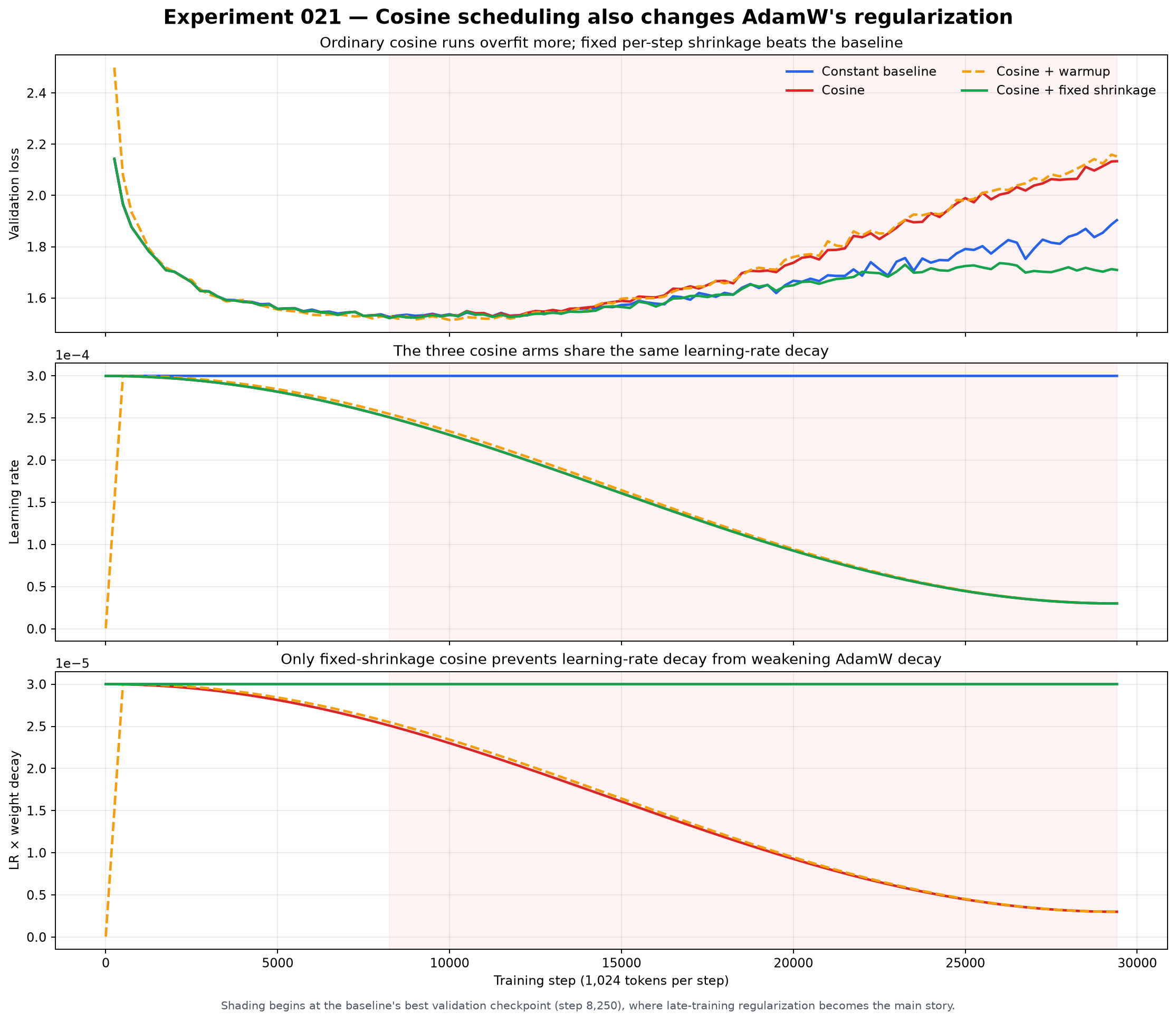
The three panels show validation loss, learning rate, and effective decay pull for each schedule. The pinned run didn’t land in the middle. It reached 1.7094, better than both the cosine run (2.1337) and the constant baseline (1.9037). Nearly all the extra overfitting was the decay following the learning rate down, and with that held fixed, the smaller late steps turned into a small independent win.
That doesn’t make cosine decay bad. Both cosine runs matched the baseline’s best validation loss; they only damaged what came after the point where I should have stopped anyway. The schedule is named after one hyperparameter but changed two, and the curve on its own doesn’t separate them. It took a third run holding the decay fixed to tell which one mattered.
SGD, Adam, and AdamW
Next I compared plain SGD, plain Adam, and the AdamW baseline at the same learning rate. SGD moves every weight by a fixed fraction of its gradient. Adam keeps running averages of each weight’s recent gradients and their size, so small but consistent gradients still get a real step and erratic ones get a cautious one. AdamW is Adam with exactly one change: where weight decay is applied.
“AdamW uses decoupled weight decay” is a sentence I’d read a dozen times and filed as a footnote. Here are both update rules side by side:
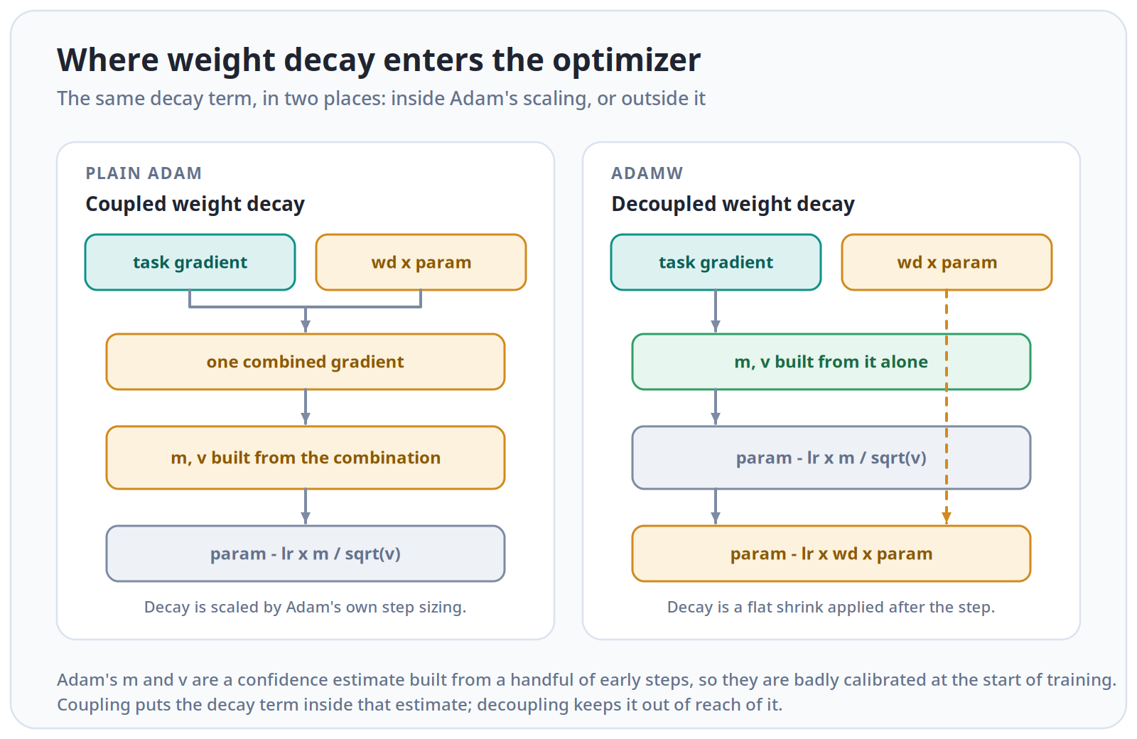
m and v are Adam’s running estimates of how
big and how consistent a parameter’s gradients have been, which it uses
to decide how large a step is safe. Coupled Adam mixes the decay into
the gradient before those estimates are built, so the decay
gets scaled like everything else. AdamW applies it separately, as a flat
shrink after the step.
I expected coupled Adam to be mildly worse. It fell apart instead.
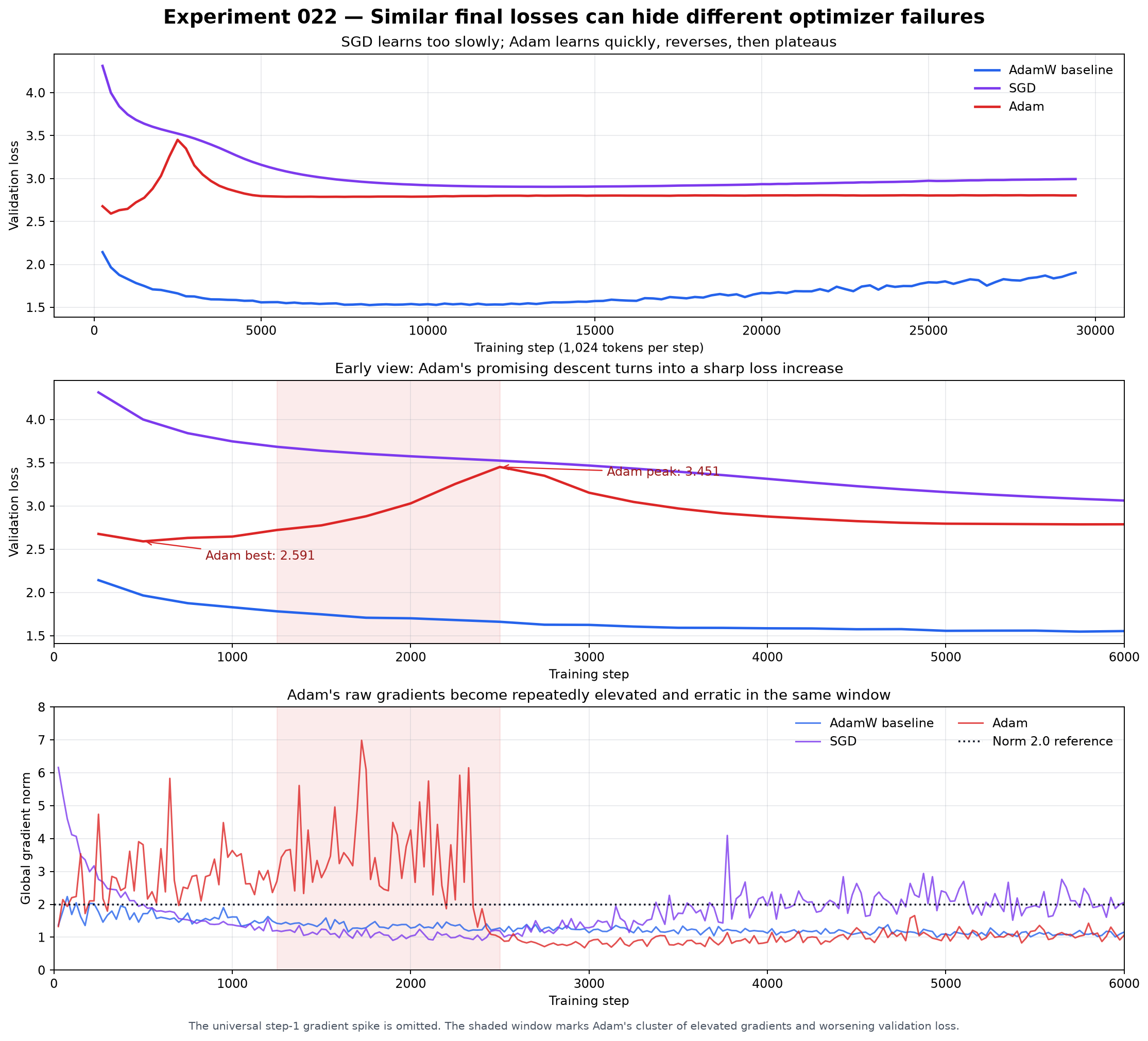
The top panel shows validation loss for the full run, the middle zooms in on the first 6,000 steps, and the bottom shows gradient norms over that window. The gradient norm is the size of a step’s gradients combined into one number, and on stable runs it sits around 1.3. For the first 500 steps coupled Adam was winning, at 2.5914. Then the gradient norm spiked to 6.10 around step 1,750, validation loss climbed to 3.4512 by step 2,500, and the run spent the remaining 27,000 steps stuck around 2.79.
Validation loss kept climbing for 750 steps after the spike ended,
then took 3,000 more to come back down. That’s momentum: m
is weighted 90% toward its previous value, so the model keeps coasting
in a bad direction after the push has stopped. Adam’s estimates start at
zero and are under-calibrated for the first few hundred steps, which
normally corrects itself. Coupling glues the decay onto the gradient
during exactly that window, so it gets amplified by the shaky early
calibration.
Plain SGD just lost, finishing at 2.9942 against AdamW’s 1.9037, with no spike. The learning rate I’d tuned for Adam is far too small for SGD. I left it untuned on purpose so the optimizer was the only change, which makes this less a verdict on SGD than a measure of how much of Adam’s value comes from per-parameter step sizes.
By final loss, those two runs look the same, both around 2.8 to 3.0, but they failed for different reasons. One was underpowered from the first step and the other destabilized and never recovered, and that difference only shows up in the early part of the curve.
Gradient Clipping
A gradient norm spiked, so the obvious next move was gradient clipping: cap the total norm at a threshold and rescale anything larger. I picked 2.0 from the baseline’s logged norms (median about 1.33, 99th percentile about 2.03) and ran it on the stable AdamW baseline as a control and on coupled Adam as the test.
The control did nothing, as intended, tracking the baseline within about 0.01 and firing on 17 of 1,178 logged steps. The test also did nothing, which wasn’t what I wanted.
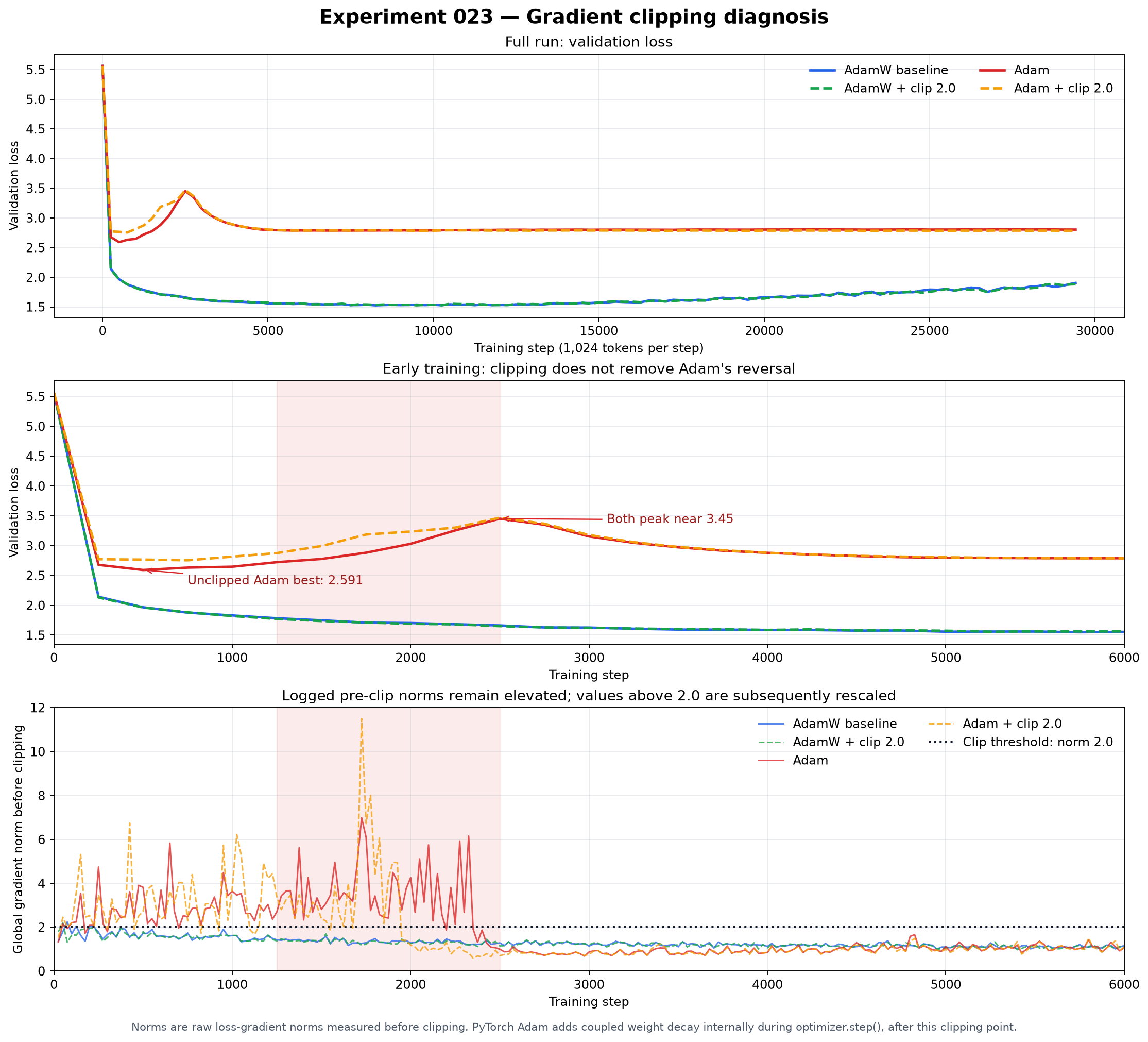
The chart shows validation loss and pre-clip gradient norms for both runs. Clipping fired 86 times on coupled Adam, concentrated right before the spike, with one raw norm as high as 11.50. The validation peak happened anyway, at 3.4683 versus 3.4512 unclipped, followed by the same plateau. The one thing clipping changed was for the worse: the fast early descent to 2.5914 vanished, because a norm cap can’t tell a large useful gradient from a large harmful one.
Reading the training loop explained why. My code calls
backward(), clips, then calls the optimizer step. But
PyTorch’s coupled Adam adds weight_decay * param to the
gradient inside that step, after my clipping. The cap applied
to the task gradient, and the quantity Adam actually used was never
capped at all.
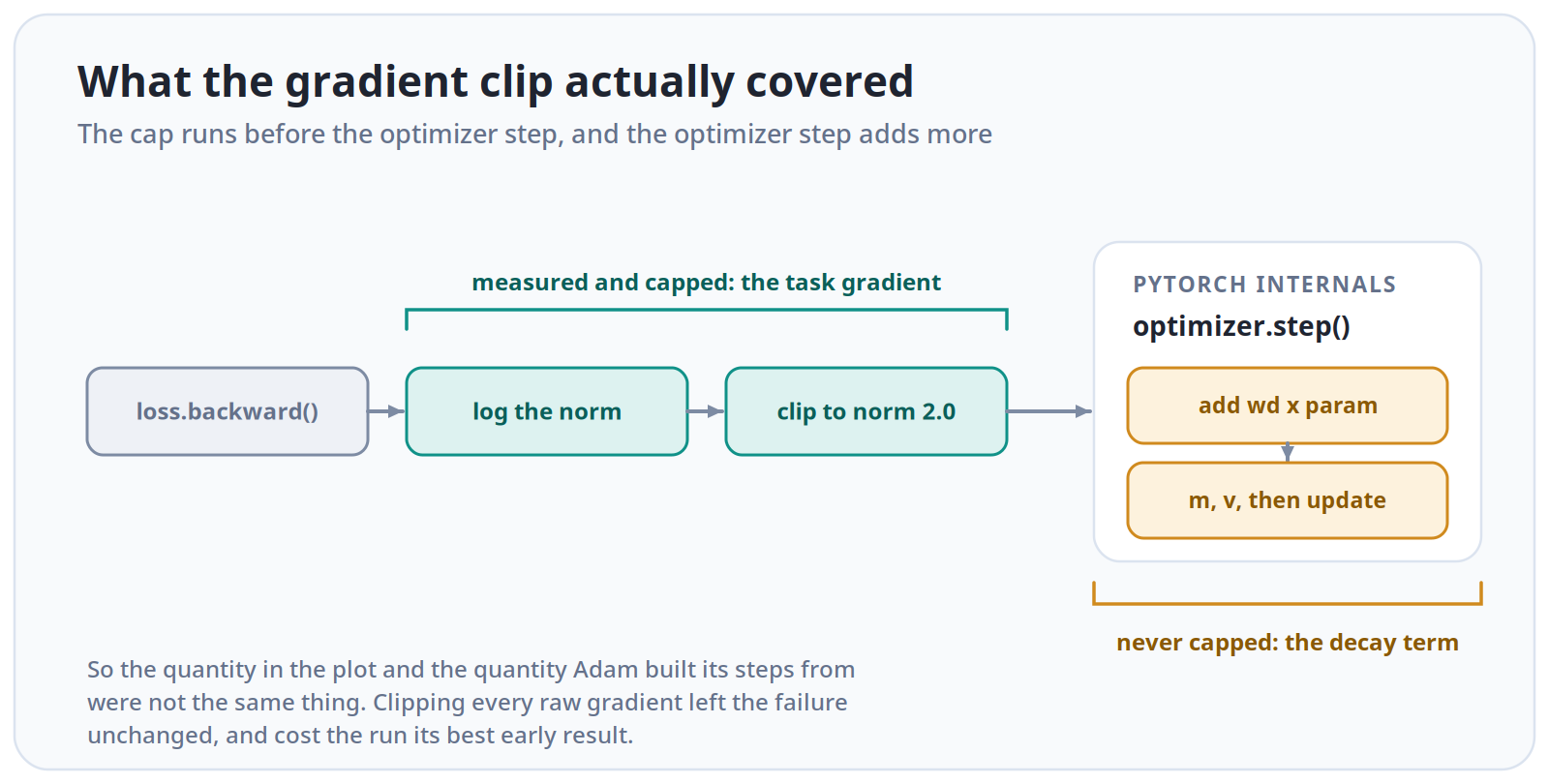
So the run rules out the raw loss gradients alone being the problem, but can’t say whether the remaining issue is a step that’s too big or one pointed the wrong way. The quantity I was clipping and the quantity the optimizer used weren’t the same, and that isn’t visible in the results, only in the order of operations in the loop.
Sweeping the Dropout Rate
Dropout randomly switches off a fraction of activations during training, so no neuron can rely on a specific partner always being there. The textbook framing is a dial with a bad end on each side: too little and the model memorizes, too much and it can’t learn.
I swept five rates from 0.1 to 0.5. Through 0.3, each step up beat the last, with best validation loss falling from 1.5260 to 1.4689, and the best checkpoint landing later each time, from step 8,250 to 28,750. At 0.4 it was a tie, 1.4694 against 0.3’s 1.4689. At 0.5 it broke: best, final validation, and final training loss all rose, which makes it real underfitting. The samples picked up small disfluencies too, like “this are not delight”.
So the sweet spot was 0.3 to 0.4, with a ceiling just past it. That turned out to be wrong.
The problem was 0.3’s best checkpoint: step 28,750 of 29,410. The curve hadn’t turned over yet, it had just run out of steps, so I reran it with twice the budget.
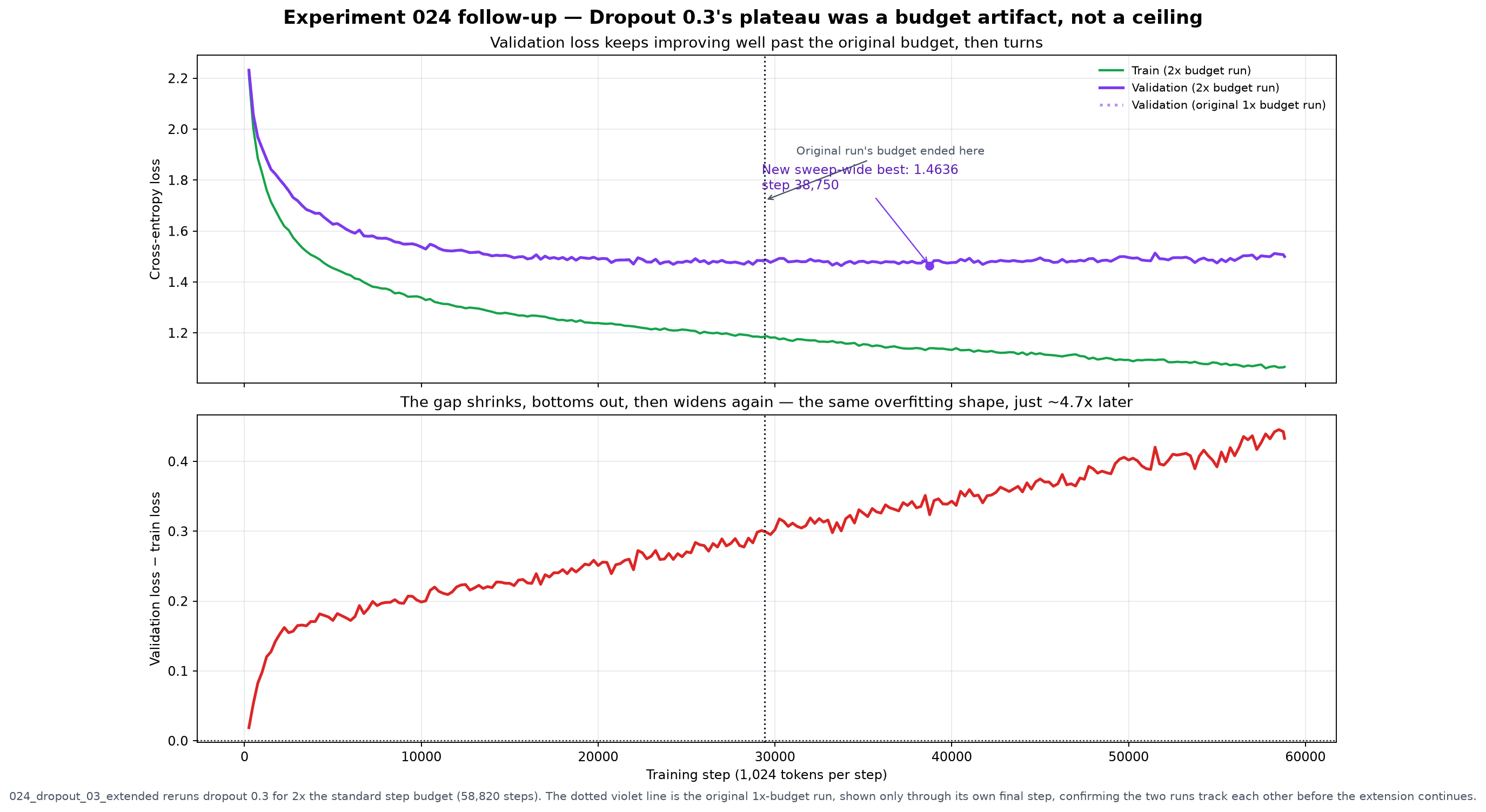
The chart shows the 0.3 run extended past its original budget. Validation loss kept improving for another 9,000 steps, reaching 1.4636 at step 38,750, better than the original sweep’s best of 1.4689. Then it climbed while training loss kept falling, the same overfitting signature as the baseline, ending at 1.4997.
Dropout didn’t remove overfitting. It postponed it, from step 8,250 to about 38,750. What I’d read as a ceiling was a curve that hadn’t turned yet, and nothing in the original plot distinguishes those two cases. When a run stops improving right at the end of its budget, the budget is the likelier explanation, and extending it is the only way to check.
Two smaller things. The generalization gap shrank at every rate, including 0.5, which was worse at both training and validation. It narrowed there because validation caught up to a degraded training loss, so read alone it would have hidden the regression. And dropout isn’t free: the cleanest timing ran at 8,703 tokens per second against the baseline’s 12,169, about 28.5% slower, just from sampling the masks.
Testing the Linear Scaling Rule
A batch is the group of sequences averaged into a single update. Mine was 16 sequences of 64 characters. The linear scaling rule says that when you double the batch, you should double the learning rate: a bigger batch gives a more reliable gradient direction, so it’s safe to move further, which makes up for getting half as many steps from the same data.
Doubling the batch to 32 at a fixed learning rate was worse at every checkpoint. Doubling the learning rate too recovered most of that and finished at 1.8895, beating the baseline’s 1.9037 with half as many steps.
The schedule experiment made me suspicious. AdamW’s shrink is
learning_rate * weight_decay, so doubling the learning rate
had also doubled the regularization, and I already knew that lever alone
could explain an improvement of about this size. So I ran an arm that
doubles the learning rate but pins the shrink back at
3e-5.
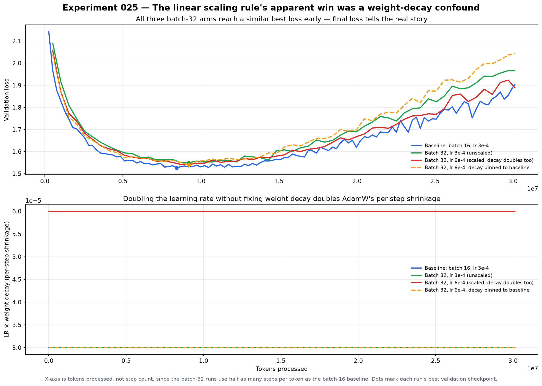
The top panel plots validation loss against tokens processed for the three batch-32 runs and the baseline, and the bottom shows each run’s effective decay pull. The pinned run came last, at 2.0429, worse than the unscaled run (1.9668) and the baseline (1.9037). It also had the lowest training loss and the widest gap: bigger steps memorized the corpus faster, and the decay pull hadn’t grown to match.
That’s close to the opposite of what I had after two arms. At this scale, the scaled learning rate mostly worked because it doubled the regularization, not because bigger steps are as good as more small ones. The rule is about step direction and says nothing about whether a fixed decay coefficient still regularizes enough.
Separately, all three batch-32 runs were about 15% faster, going from the baseline’s 12,169 tokens per second to around 14,000. That came from spreading per-step overhead over more tokens. That part holds regardless of the loss.
Mixed Precision with bfloat16
The last experiment was mixed precision: run the forward pass in bfloat16 and keep the weights, gradients, and optimizer state in float32. bfloat16 has much less precision than float32 (7 bits of mantissa instead of 23) but the same range, so it doesn’t need float16’s overflow handling. Rounding is harmless in forward-pass results that are thrown away after one step, but not in weights and running averages that accumulate tiny changes over tens of thousands of steps.
Before running it, I checked lscpu for
avx512_bf16. Without it, PyTorch emulates bfloat16 in
software, and I’d have measured a slowdown and drawn the wrong
conclusion.
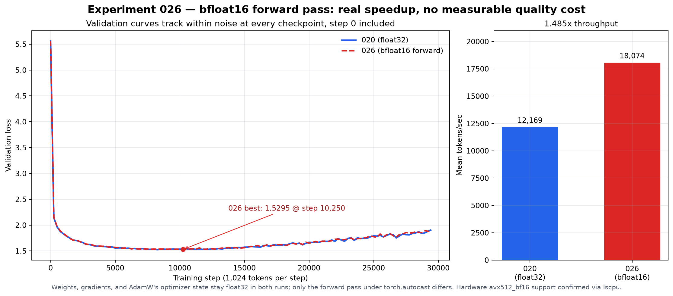
The chart overlays the bfloat16 and float32 validation curves. Throughput went from 12,169 to 18,074 tokens per second, 48.5% faster, and the curves are indistinguishable: 1.5296 best against 1.5260, 1.8890 final against 1.9037.
My favourite number is from step 0, before any training: 5.5612 against 5.5614. Same weights, same data, one forward pass in two precisions. That’s the size of what bfloat16 actually changes. After five experiments where the appealing number had something hiding behind it, this one just worked as advertised.
Swapping the MLP for SwiGLU
Later, after the training-systems work in the next post, I came back to this baseline for one change that is not a training decision at all: the feed-forward layer. It is an architecture change, so it would have belonged in the architecture post, but that post was written before this baseline existed, and a baseline that overfits on schedule is exactly what I wanted to test it against.
Every transformer block does two things. Attention lets each character’s vector pull in information from earlier characters. Then a small two-layer network, the MLP, processes each character’s vector on its own. Mine expanded each 256-number vector to 1,024 numbers, passed them through GELU, and projected back down to 256. You can picture those 1,024 middle numbers as feature detectors. Each one measures how well the input matches its pattern, GELU switches it roughly off if the match is negative, and whatever survives gets written back out, scaled by how strongly it fired.
The limitation is that one number does two jobs. The same score decides whether a detector fires and how much it contributes. SwiGLU, from Noam Shazeer’s 2020 paper GLU Variants Improve Transformer and now the default in the Llama family, splits those jobs. Two separate projections read the input: one passes through SiLU (a curve almost identical to GELU) and acts as a dimmer, and the other carries the signal. The two are multiplied together element by element before the projection back down. The curve barely changes. What’s new is that multiplication, which lets a single channel express “this pattern, but only in that context.”
Three matrices instead of two cost 50% more parameters at the same width. This time I asked what else the change was attached to before running it, and shrank the middle from 1,024 to 683. That’s the same two-thirds reduction the paper made, and the closest a whole number gets to an exact match: 5,839,104 parameters against 5,837,056, a difference of 0.035%.
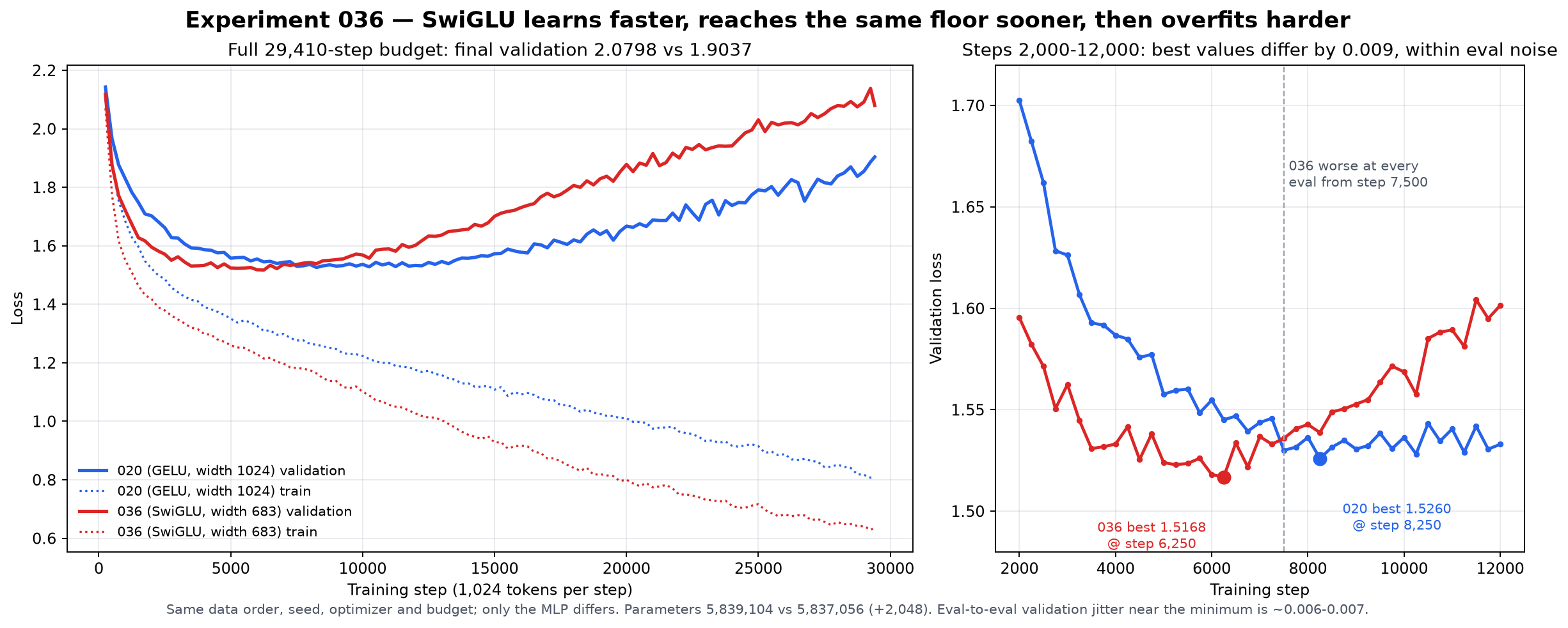
My prediction was a better best validation loss, with overfitting setting in earlier. Only the second half held up. SwiGLU’s best was 1.5168 at step 6,250, against 1.5260 at step 8,250. That’s lower, but the validation loss already wobbles by 0.006 or so between one check and the next near the minimum, so 0.009 from a single run each is a tie. After step 7,500 it was worse at every single check, and it finished at 2.0798 against 1.9037.
What SwiGLU really changed was speed. It reached every validation milestone in 55 to 60 percent of the steps the GELU model needed: 1.60 at step 2,000 instead of 3,500, and 1.55 at step 3,250 instead of 5,750. Then it hit the same floor and started memorizing sooner than the GELU model did.
That fits the dropout result more than it contradicts the paper. Shazeer measured at equal training steps on a corpus so large that nothing is ever seen twice, and there, learning more per step simply is a better model. Here the model reads the same megabyte of Shakespeare thirty times, and the limit was never the MLP. It was how much there is to learn from that megabyte before the only thing left is memorizing it. Dropout pushed that point later, and SwiGLU reached it sooner. Neither moved the floor. What an architectural improvement buys depends on what is limiting the model, and here that was the data.
Where I Ended Up
I can now explain what a cosine schedule does to weight decay, why
coupled and decoupled decay aren’t the same thing, what dropout buys and
costs, and why I check lscpu before believing a
speedup.
The more useful takeaway was that the mistake was the same every time. A schedule that changes the learning rate also changes the regularization. A doubled learning rate doubles it too. Clipping before the optimizer step doesn’t cover what the step adds. A sweep with a fixed budget measures the budget as much as the setting. Each time I changed one named thing and something unnamed came along, and twice the result flipped once I held it still.
None of those results looked broken; they looked like findings. I only caught them because the numbers were slightly better than I expected and the control run was cheap. So the habit I’m keeping is to ask what else a setting is arithmetically tied to before running the comparison, and to treat a better-than-expected result as a possible confound. I checked that twice here and found a confound both times.
Next I looked at training as a system rather than a set of settings: where the time goes in a step, whether a run can be stopped and resumed without changing what it learns, what happens when the numbers go bad, where the memory goes, and how much throughput was sitting in the CPU thread count all along.