My last post changed the transformer one piece at a time, but all of those were changes to parts I had already built. Mixture of Experts was the first thing I added that was genuinely new to the model.
It also had the biggest gap between its reputation and its size as an idea. Several frontier models are built this way, and the descriptions I’d read made it sound like a fundamentally different architecture. Implementing it took about eighty lines.
What I didn’t expect was that the two most useful things I learned would have almost nothing to do with Mixture of Experts. Both were about how convincingly a broken component can imitate a working one.
Four MLPs Where There Was One
Each transformer block in my model ran attention, then a single MLP shared by every token. A Mixture of Experts layer replaces that MLP with several, plus a small learned router that picks which one each token uses.
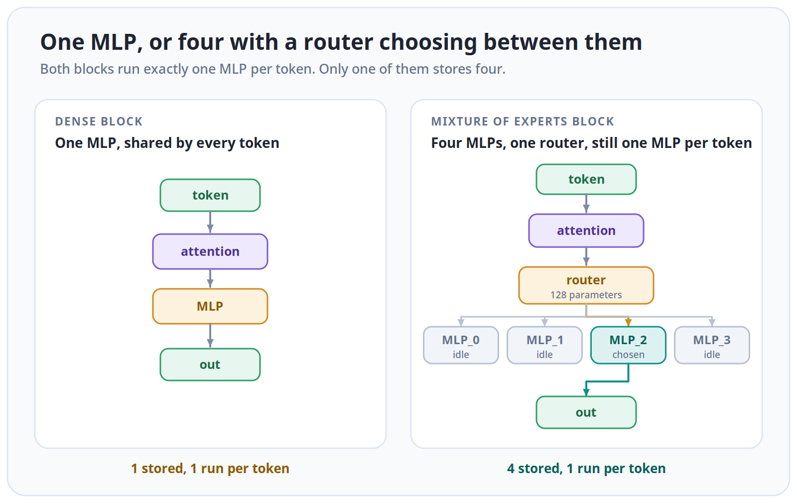
I used four experts and picked one per token. The dense model stores one MLP and uses one. The Mixture of Experts model stores four and still uses one. That’s the whole trade: a bigger model that costs about the same to run, like a hospital with four specialists instead of one generalist, where each patient still sees exactly one doctor.
I had two details wrong before implementing it. Routing is per token, not per sequence, so a batch of 64 sequences of 16 characters means 1,024 routing decisions, not 64. And every block has its own router and experts, so a character can go to expert 2 in the first block and expert 0 in the second.
The router is deliberately tiny: one linear layer from the 32-value token representation to four scores. That’s 128 of the model’s 76,608 parameters. Those 128 numbers are four directions in the embedding space, one per expert, and a token’s score for an expert is its dot product with that direction. Training the router means learning how to carve up the space.
Turning the Dispatch Loop Inside Out
The obvious implementation loops over tokens and runs each one through its expert. That’s 1,024 tiny calls per layer, which wastes hardware built for large matrix multiplications. The fix is to turn the loop inside out: loop over experts and gather their tokens. Four calls instead of 1,024.
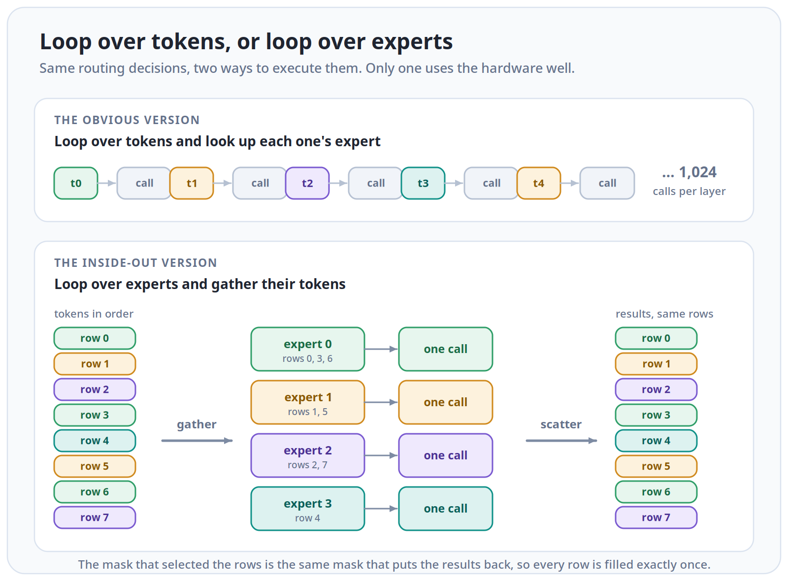
Every result has to return to its original row, because the next layer reads tokens in order. So the layer starts with a zero tensor, builds a mask of which rows chose the current expert, gathers those rows, makes one batched call, and scatters the results back through the same mask. While writing it, the masking felt like bookkeeping. Reading it as “loop over experts, gather their tokens” made it look like the only sensible way to batch the thing.
This is also what sparse actually means here. Tokens that didn’t choose an expert never enter its matrix multiplication. It isn’t computing all four and discarding three.
A Router That Never Trained
My first working version trained fine. The loss fell, and the routing distribution moved for about 500 steps and then went flat. I wrote that down as the router settling into a stable partition.
It hadn’t settled. It had never moved at all. The dispatch computed the router’s weight like this:
top_k_weights, top_k_indices = torch.topk(router_logits, k, dim=-1)
top_k_weights = F.softmax(top_k_weights, dim=-1)
The softmax runs after the selection. With one expert selected, it
gets a list of one element, and a softmax over one element always
returns 1.0. That’s a constant, with zero derivative. Since
topk isn’t differentiable either, the router received no
gradient at all.
Printing the gradients settled it. With one expert selected, all 128 router gradients were exactly zero. With two selected, they were a healthy 9.322e-03. After the fix, one expert gave 2.771e-03. The expert MLPs trained normally the whole time, which is why the loss curve never looked wrong.
The fix is to apply the softmax over all four scores before selecting, which is the Switch Transformer formulation and exactly why Switch can train with one expert per token:
router_probs = F.softmax(self.router(flat), dim=-1)
top_k_weights, top_k_indices = torch.topk(router_probs, k, dim=-1)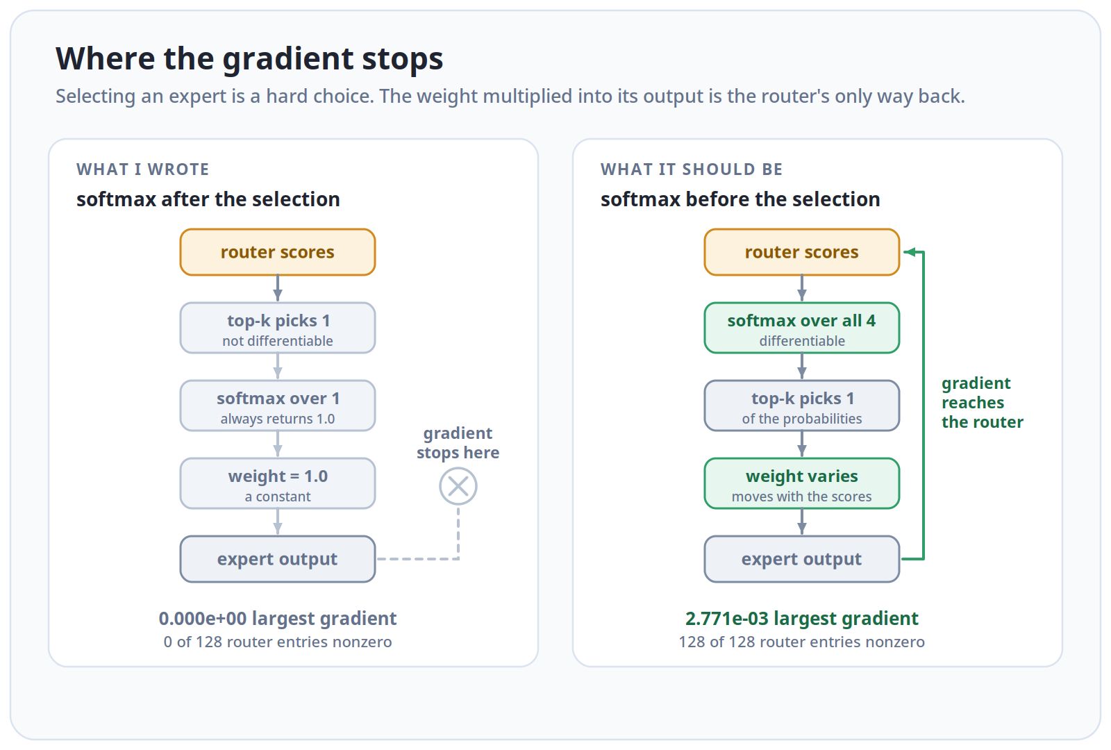
This also answered a question I’d parked: why multiply the expert’s output by its weight at all, when with one expert that weight is about 1.0? Its job isn’t numerical. Picking an expert is a hard choice with no dial attached, so that multiplication is the only place the router’s output enters the computation, and the only route a gradient has back to it.
Turning the router on was worth 0.030 validation loss (1.8048 to 1.7745, same config and seed). Real but modest, which suggests most of what Mixture of Experts bought me here came from extra capacity, not clever routing.
What stays with me is how complete the story around the bug was. The loss fell to near my best. The routing chart showed four experts with visibly different usage, exactly what specialization should look like. I was looking at the random initialization, unchanged after 5,000 steps. Even the early drift had a different explanation: token representations sliding around under a partition that never moved.
Checking took one command. Print the gradient and see whether it’s zero.
Sparse Does Not Mean Fast
I had absorbed the idea that Mixture of Experts gives you capacity for free. Counting arithmetic supports that. The clock doesn’t. The dense run took 73.8 seconds for 5,000 steps, and the one-expert Mixture of Experts run took 81.0.
Memory is the obvious cost. All four experts stay resident, so the model holds 76,608 parameters to do the arithmetic of about 27,200. That’s the same ratio that shapes real deployments, where Mixtral 8x7B loads around 47 billion parameters to compute about 13 billion per token.
The cost I hadn’t considered is data movement. Gathering and scattering rows is pure movement with no arithmetic, and four roughly 250-row matrix multiplications are less efficient than one 1,024-row one. At my scale that’s a few seconds. At real scale, where experts live on different machines, the same shuffling becomes network traffic and the dominant engineering problem.
Going to two experts per token made this concrete. Parameters stayed at exactly 76,608, but each token now passed through two experts. Training time went from 81.0 to 123.5 seconds, 52.5% slower, for a validation improvement of 0.0133, from 1.7745 to 1.7613. Parameter count describes what’s stored. Experts per token describes what’s run. I had been treating those as one number.
The runtime didn’t double because attention, normalization, embeddings, loss, and the optimizer still cost what they did before. Doubling one part and seeing 52.5% more runtime tells you roughly how much that part owned.
Reading My Own Routing Chart Wrong
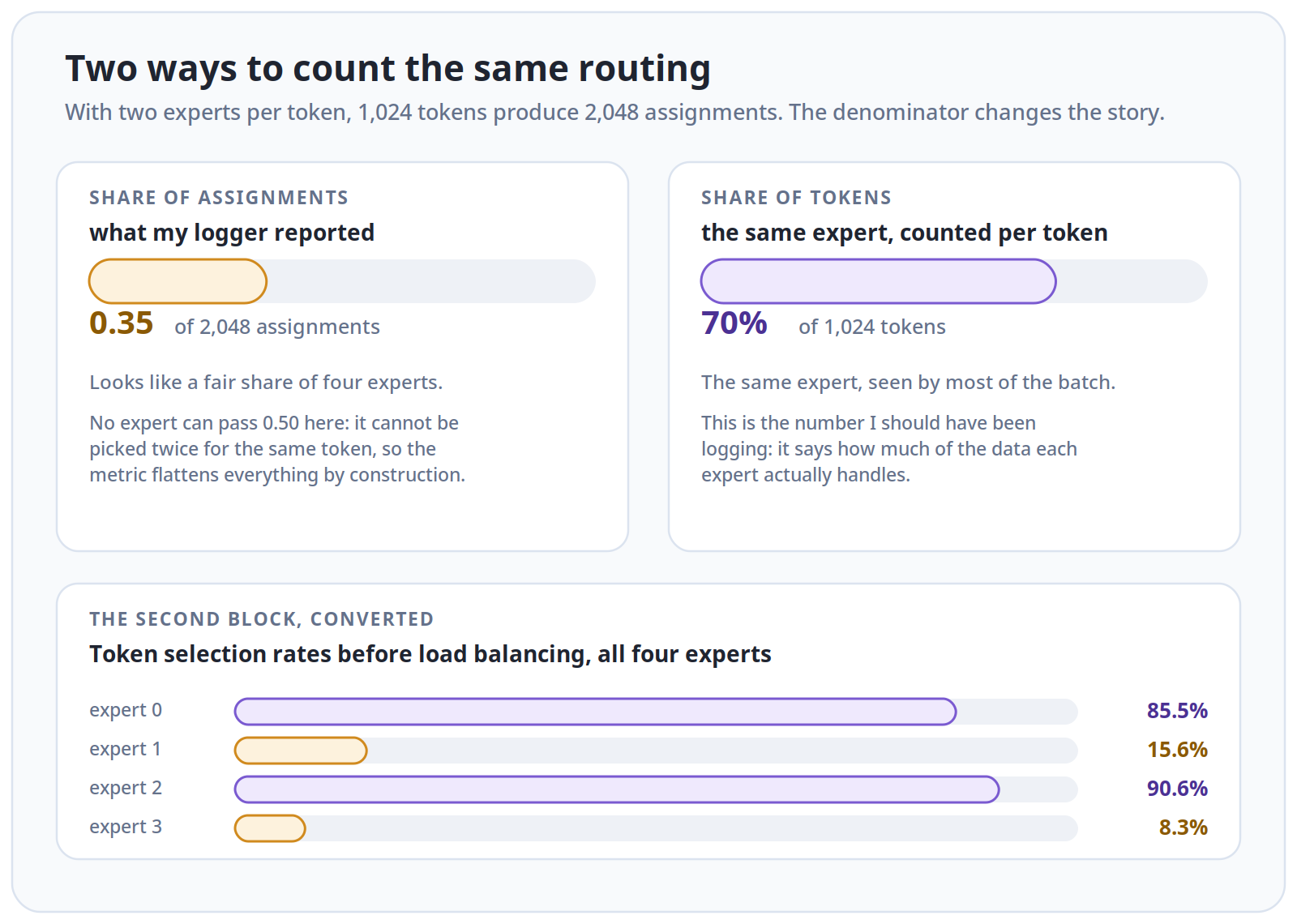
With two experts per token, my routing chart looked healthy. The first block’s experts sat at roughly 0.24, 0.27, 0.27, and 0.22 of assignments.
That evenness was partly an artifact of how I measured it. I divided each expert’s count by total assignments, but with two picks from four, no expert can exceed 0.50, and 0.35 of assignments actually means being picked for about 70% of tokens. Converting to the share of tokens selecting each expert, which is what I should have logged in the first place, the second block was badly lopsided: two experts at 85.5% and 90.6%, one at 8.3%.
Why Routers Collapse
The router couldn’t have known better, because balance appears nowhere in the loss. It’s trained only on whether the next character was predicted well.
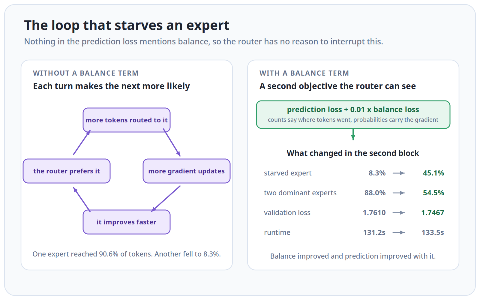
There’s also a feedback loop pushing the wrong way. An expert that gets more tokens gets more updates, improves faster, and attracts more tokens. My run didn’t start with a starved expert. The concentration built up over training.
The standard fix adds a term that makes balance visible to the router:
balance loss = number of experts
             x sum(assignment share x mean router probability)

total loss = prediction loss + 0.01 x balance loss
It needs both parts. The hard assignment counts describe where tokens actually went, but you can’t get a gradient through the selected indices, so the soft router probabilities carry the signal back.
The effect of a 0.01 weight was bigger than I expected. The starved expert went from 8.3% of tokens to 45.1%, and the two dominant experts fell from a combined 88.0% of assignments to 54.5%, for 1.7% more runtime. Validation loss improved too, from 1.7610 to 1.7467. I expected to pay something for forcing the routing flatter. That I didn’t suggests the lopsidedness was the feedback loop running away, not a partition worth keeping.
The loss curves below compare normalized top-2 routing with and without the balance term. They’re worth looking at because they’re so boring.
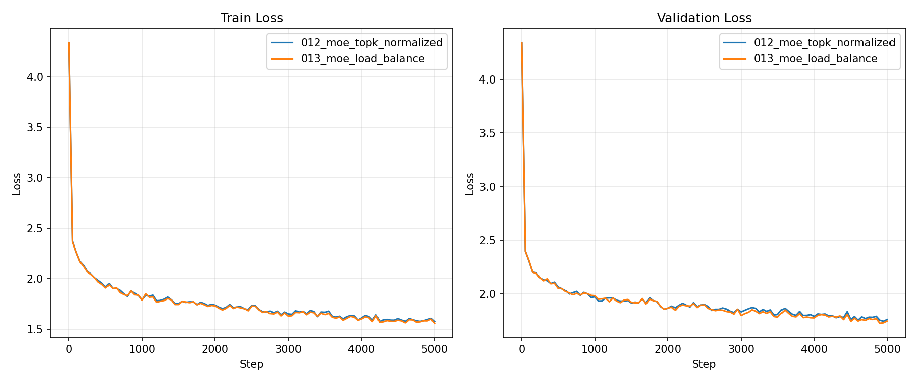
Almost the only visible difference is a slight separation over the last thousand steps. Underneath, one expert went from nearly unused to carrying a normal share of the traffic. The number I was ranking runs by shows almost none of what the experiment was about.
Balanced doesn’t mean identical: the second block still picked one expert for 62.1% of tokens and the others for 45 to 47%. And at this size, balancing isn’t doing its production job. My experts have unlimited capacity and run one after another, so here it just keeps neglected experts learning. In a real deployment, with experts in parallel on different devices and limited capacity each, it’s an operational requirement.
What It Cost and What It Bought
Mixture of Experts wasn’t worth it at this scale. My best run reached 1.7467 with 76,608 parameters. Extending the context window from 16 to 32 characters took the dense model from 1.848 to 1.7789 with 29,760. That’s 2.6 times the parameters, and slower steps, for about 0.03 over a much simpler change.
That’s not an argument against the technique. It says my model was limited by context, not capacity, and something that works at 47 billion parameters is under no obligation to help at 76 thousand. I’d rather have this result than a flattering one. It separates knowing how a mechanism works from knowing when to reach for it.
A Failure I Could Rule Out
Every run here generated nothing but newlines, the same degenerate behavior I hit with rotary positional embeddings last time. Better validation loss didn’t help, which fits: validation never asks the model to consume its own output.
The bug did give me one new piece of evidence. The broken-router and fixed-router runs produced byte-identical output, so routing can’t be the cause, which points back at the positional encoding. The accidental bug ended up serving as a control for a different one.
Where I Ended Up
I can now write a sparse Mixture of Experts layer, explain why the selected weight is multiplied in, and say why the balancing term is necessary. I also have a case where the technique didn’t pay off, and a reason why.
The part I expect to keep is smaller. Twice, something was broken in a way the validation loss couldn’t show me: a router with no gradient, and a routing chart whose balance came from dividing by the wrong number. Both took one command to expose once I looked at the component itself.
So I’ve started asking whether a thing is running before asking how well it ran, and logging the two things that would have caught these: each component’s gradient size, and the share of tokens choosing each expert. Both are one line.
Next I left the architecture alone and changed how the model trains: learning rate schedules and weight decay, why Adam and AdamW differ, how dropout delays overfitting without preventing it, and whether mixed precision makes training faster without changing what the model learns.