My last post ended with a small GPT that I could follow from tokenization through backpropagation. I knew what the context window, embedding size, attention heads, layers, activation function, and positional embeddings were supposed to do, but I had little intuition for what would happen if I changed one of them.
So that became the next set of experiments. I kept the training loop fixed and changed one architectural choice at a time. The goal wasn’t to find the best small model. It was to connect each piece of the implementation to the behavior it produced.
The experiments ran on Tiny Shakespeare, a character-level dataset with a 65-character vocabulary. The children’s-book dataset from the last post was too easy: most changes either did nothing or overfit. Shakespeare had enough dialogue, names, and punctuation to expose differences.
The baseline had a context length of 16 characters, 32 embedding
values, 4 attention heads, and 2 layers. It had 29,248 parameters and
reached a validation loss of 1.848. Its samples picked up some of the
source’s formatting but fell into loops like the shall,
which left plenty of room for changes to show.
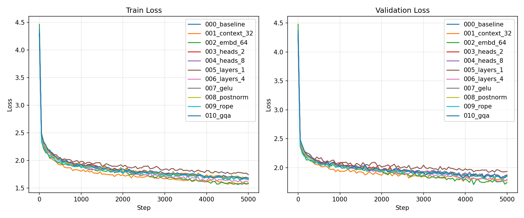
The plot shows validation loss over training for each variant. Some changes separated early and stayed separated, while others landed right on top of the baseline, which told me whether a final difference reflected the whole run or just the last checkpoint.
Making the Model Larger
Doubling the context length from 16 to 32 improved validation loss from 1.848 to 1.779. Seeing further back seemed to help with dialogue turns and character names. Training took about 1.6 times as long even though the parameter count barely changed, because attention had more pairs of positions to compare. This was the first time the context window felt like more than a config value: the model cannot use a clue it was never allowed to see.
Doubling the embedding size from 32 to 64 gave the biggest improvement, from 1.848 to 1.745, while growing the model from 29,248 to 107,648 parameters. The same change had mostly caused overfitting on the simpler dataset. Whether a model is too small or too large isn’t a property of the model alone. It depends on what the data asks of it.
Depth helped less. One layer made loss worse, from 1.848 to 1.935, and four layers improved it from 1.848 to 1.800 at roughly twice the training time. I’d heard width and depth described as two kinds of capacity, and this made it concrete. Width gives each token more room to describe things. Depth gives the model more passes to refine those descriptions. They don’t buy the same thing or cost the same.
What Is an Attention Head For?
I tried 2 and 8 heads with the embedding size fixed at 32. Since the embedding is split between heads, this changes the size of each head rather than adding features. With 2 heads (16 values each) loss was 1.874. With 8 heads (4 values each) it was 1.867. Neither beat the baseline’s 1.848, and the parameter count didn’t change.
I used to think of more heads as simply more parallel attention patterns. That is true, but more heads also means each one gets a smaller slice of the same budget. The head count can’t be interpreted apart from the embedding size, and that turned out to be a recurring theme: what looks like one isolated knob is usually tied to tensor shapes and costs elsewhere in the model.
ReLU and GELU
Swapping ReLU for GELU changed validation loss from 1.848 to 1.846, a tie. I expected GELU’s smooth transition around zero to matter more in a larger or deeper model, and this didn’t contradict that. It was a useful non-result: a component can be in every modern LLM for good reasons that just aren’t visible at this scale.
Moving Normalization Around
I compared the baseline’s pre-norm structure with the post-norm structure from the original Transformer paper. Pre-norm normalizes the input to each branch:
hidden = hidden + attention(norm(hidden))
hidden = hidden + mlp(norm(hidden))
Post-norm normalizes the result of the residual addition:
hidden = norm(hidden + attention(hidden))
hidden = norm(hidden + mlp(hidden))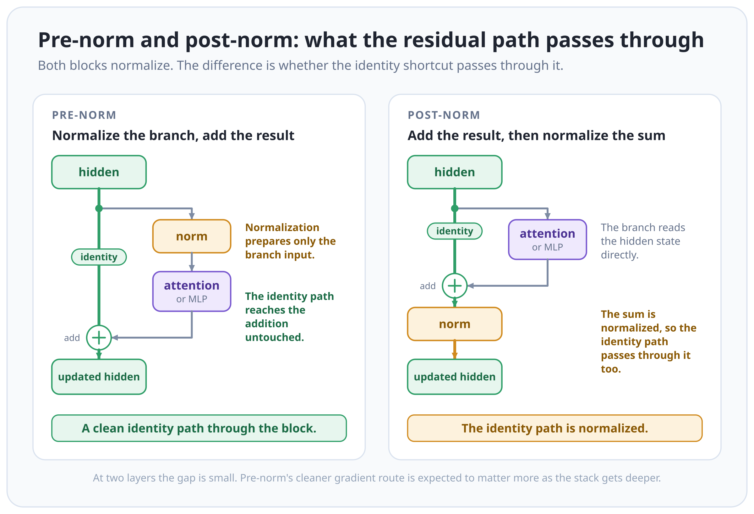
At two layers the results were nearly identical (1.857 vs 1.848). The code made the usual “pre-norm is more stable” explanation click, though. The residual connection is supposed to be an identity path that each block adds a small correction to. Pre-norm leaves that path untouched. Post-norm pushes it through normalization at every block, so gradients lose their clean route through a deep stack. Two layers just aren’t enough for that to show up.
I also noticed my implementation had an initial normalization left over from the scalar model and no proper final normalization. A good reminder that comparing two named choices doesn’t mean either one is a clean implementation.
RoPE Was the First Real Surprise
The baseline used learned absolute position embeddings: a learned vector per position, added to the token embedding at the start. For RoPE, I dropped that table and instead rotated pairs of dimensions in the query and key vectors inside each attention layer, by angles that depend on position. The difference came down to this:
- Learned position embeddings tell a token where it is before attention begins.
- RoPE makes the comparison between two tokens aware of their relative distance.
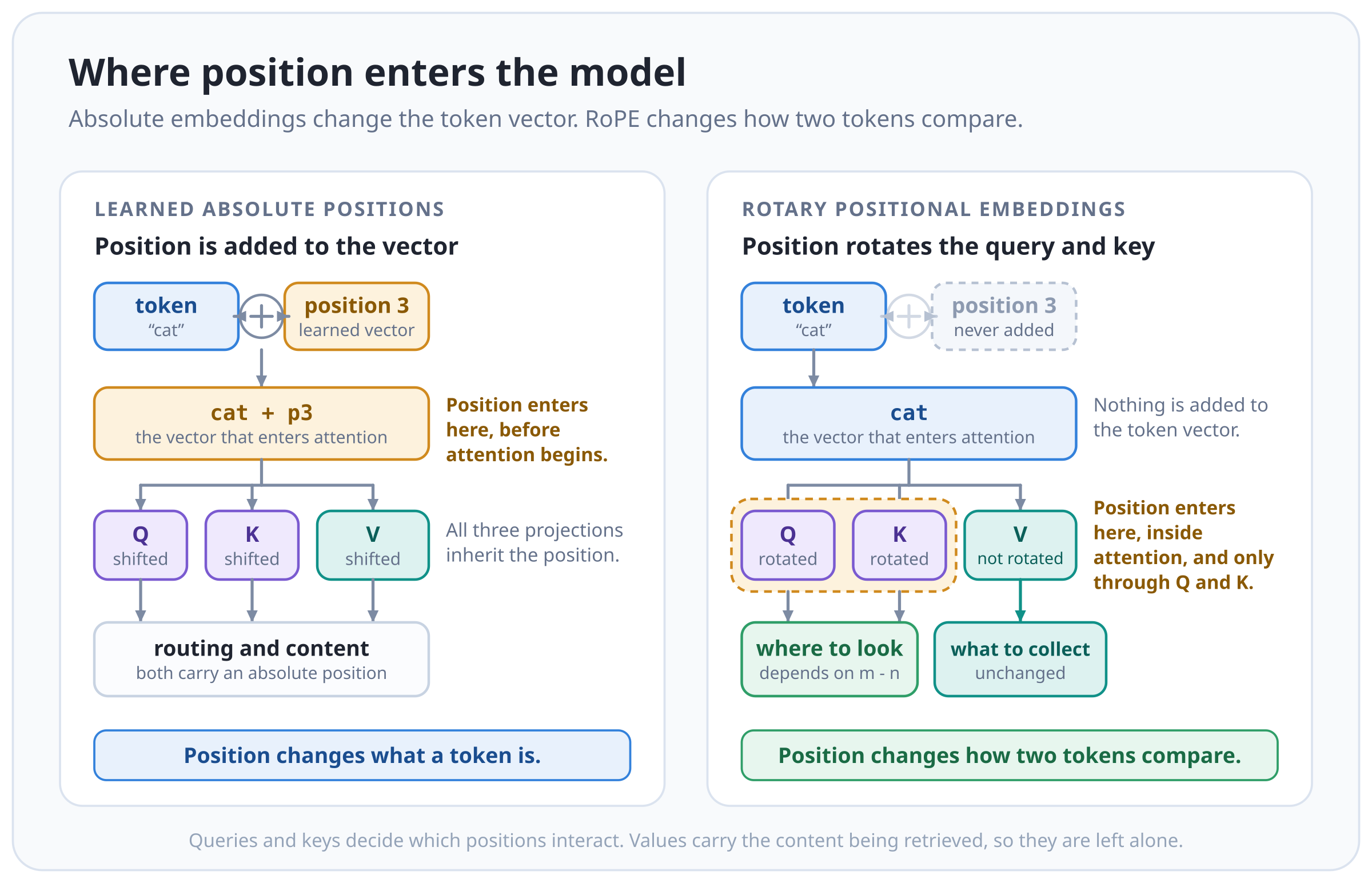
Values aren’t rotated. Position affects which tokens get looked at, not the content that gets retrieved.
RoPE reached 1.844, essentially the baseline’s 1.848. With a context of 16, a learned table can memorize every position it needs, so I didn’t expect much. The surprise was the generated sample: nothing but newlines.
It took me a while to work out why. During training the model sees varied text, so even if attention routing changes, the values it retrieves differ. During greedy generation, this tiny model fell into a newline loop. Once every position held the same character, every value vector was the same, so no matter where the rotated queries and keys pointed, attention returned the same content. Each newline reinforced the next.
This was the most important evaluation lesson I took away. Validation loss is teacher-forced: the model always gets the correct previous characters. During generation it has to live with its own outputs, and a model can look fine in one setting and fail in the other. I don’t read this as RoPE being bad for language models, since the tiny model, short context, and greedy decoding all contributed. I read it as generation samples being necessary evidence.
GQA and the Difference Between Training and Inference
Standard multi-head attention gives each query head its own keys and values. Grouped-query attention keeps a query per head but shares keys and values within groups. In my run, two query heads shared one key/value pair and the other two shared another. Each head can still ask a different question of the same shared keys and values, like several historians researching different topics in the same library.
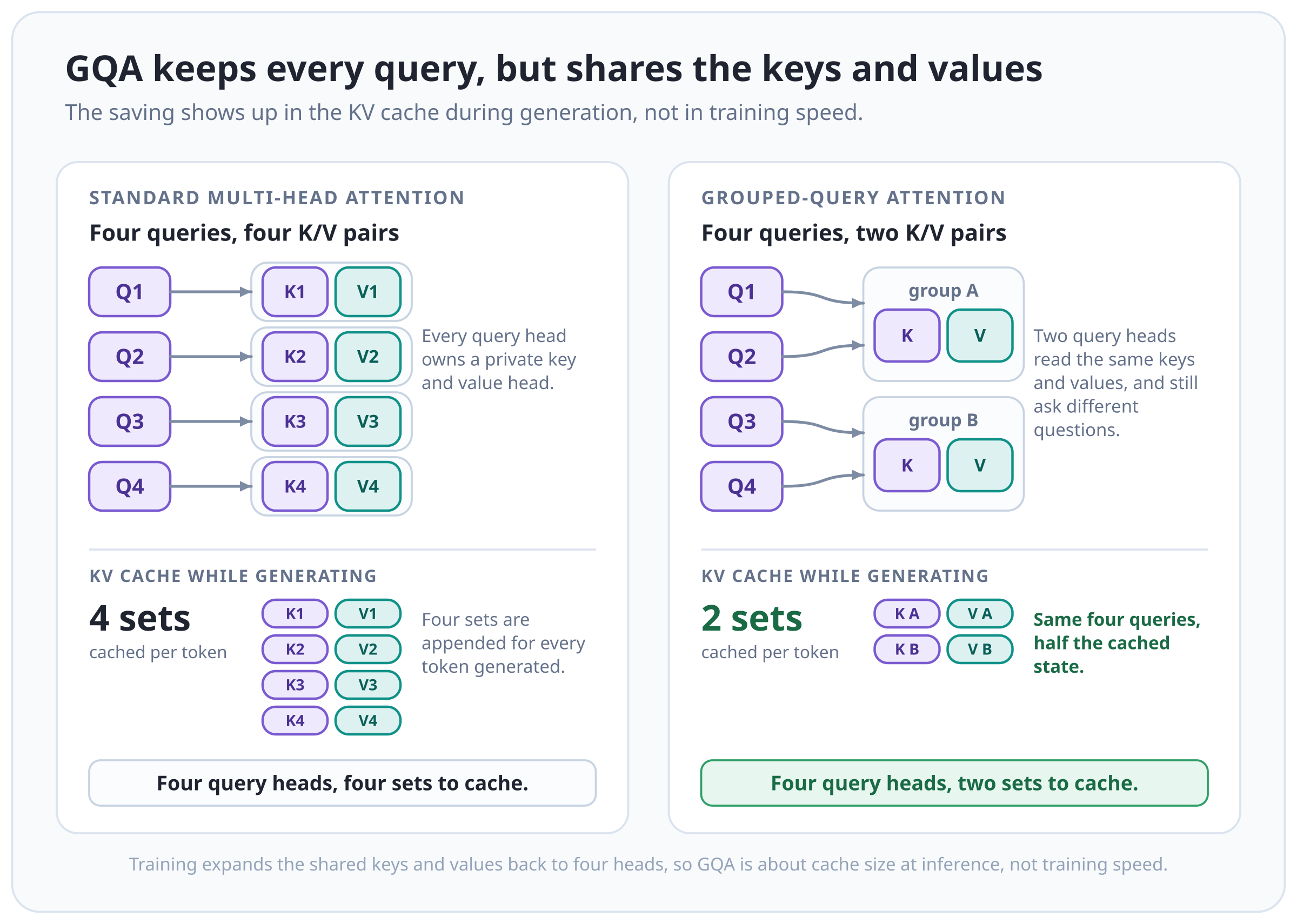
The code confused me at first. The key and value projections are narrower than the query projection, so they produce two heads where the query produces four:
# n_embd 32, n_head 4, n_kv_head 2, head_dim 8
self.query = nn.Linear(n_embd, n_head * head_dim, bias=False)     # 32 -> 32
self.key = nn.Linear(n_embd, n_kv_head * head_dim, bias=False)    # 32 -> 16
self.value = nn.Linear(n_embd, n_kv_head * head_dim, bias=False)  # 32 -> 16
Then the forward pass expands them straight back to four:
query = self._split_heads(self.query(hidden), n_head)     # (B, 4, T, 8)
key = self._split_heads(self.key(hidden), n_kv_head)      # (B, 2, T, 8)
value = self._split_heads(self.value(hidden), n_kv_head)  # (B, 2, T, 8)

# A KV cache would store key and value at this size, before the repeat.
n_rep = n_head // n_kv_head
key = key.repeat_interleave(n_rep, dim=1)                 # (B, 4, T, 8)
value = value.repeat_interleave(n_rep, dim=1)             # (B, 4, T, 8)
That expansion looked like undoing the whole point. The repetition just keeps the attention tensor shapes unchanged. The real benefit is at inference, where previous keys and values are stored in a KV cache and GQA stores fewer of them.
On this model, GQA saved about 2,048 parameters, made loss slightly worse (1.848 to 1.869), and trained at the same speed. With 32 embedding values and a context of 16, the KV cache was too small for the savings to matter, while the lost capacity was noticeable. That separated two questions I’d been blending together: does this train better in a tiny benchmark, and does it make a large model cheaper to serve? GQA is answering the second one.
What Changed in My Mental Model
No single architecture came out on top. The wider model did best on this dataset, but that wasn’t the point. I stopped treating architecture diagrams as a list of interchangeable parts with obvious effects. Most changes turned out to be trade-offs tied to shapes and costs elsewhere, and some, like GELU and normalization placement, probably matter at scales I never reached.
I also got more careful about what a result actually supports. A flat curve could mean a change does nothing, or that the model is too small for the effect to appear. Parameter count and training speed can completely miss an inference optimization like GQA. And validation loss isn’t the final judge: RoPE’s generated text exposed a failure the loss hid.
Now when I look at a transformer config I ask more specific questions. What can each position see? How is the representation budget split between heads? Is a change meant to improve capacity, optimization, throughput, or inference memory?
Every experiment here changed a part I had already built. Next I added one I hadn’t: a Mixture of Experts layer, which swaps the single MLP in each block for several, plus a small router that picks which one each token uses.