Learning How GPTs Work by Building One from Scratch

I’ve wanted to properly understand how GPTs work for a while. I knew most of the vocabulary: embeddings, attention, softmax, residual connections. I had used PyTorch and built a small neural network from scratch a few years ago. But if I tried to follow the full path from input text to a weight update, my understanding got hand-wavy pretty quickly.

So I went back to the beginning. I worked through Ian Bull’s LLMs, the Hard Way, which builds a small GPT in TypeScript without a machine learning framework. I followed the same path in Python, first with a version where every value in the model was an individual scalar, then with a normal PyTorch implementation.

The model I ended up with generated simple sentences like the sheep is by the tent. That isn’t useful on its own, but model quality wasn’t the point. I wanted to be able to look at a GPT implementation and understand why each part was there and what happened during training.

Starting with Individual Numbers

I started with a simple word-level tokenizer that split sentences on spaces, assigned a number to each word, and added a special token to mark the start and end of a sentence.

I had always thought of tokenization as preprocessing that happens before the interesting work. The later fine-tuning section showed me it’s tied directly to what the model learns. If cat is token 89, then row 89 of the embedding table learns the representation for cat, and output 89 is the model’s score for generating cat. Rebuild the tokenizer so 89 means where, and you’ve just scrambled the meaning of the model’s inputs and outputs. Obvious once it’s laid out, but I hadn’t thought it through before.

Next I implemented a small Value class. Each Value held one number, its gradient, and a record of how it was calculated. Operations like addition, multiplication, powers, exponentials, and ReLU all returned another Value. There were no tensors: a vector was a list of Value objects and a matrix was a list of those lists. Slow, but I could inspect every calculation the model made.

Finally Understanding What backward() Does

Autograd was the first part that really changed my understanding. I knew what backpropagation did at a high level, but not how PyTorch kept track of it all automatically.

In the scalar version, every operation records how to pass a gradient back to its inputs. Addition passes it to both. Multiplication scales it for each input by the other input’s value. ReLU passes it through or blocks it depending on whether the input was positive. Here’s multiplication, with some type details removed:

def __mul__(self, other):
    output = Value(self.data * other.data)
    output._parents = (self, other)

    def backward():
        self.grad += other.data * output.grad
        other.grad += self.data * output.grad

    output._backward = backward
    return output

Calling backward() starts at the loss and walks these recorded operations in reverse. Each one only knows its own small derivative rule, and chaining them together gets the gradient back to every weight.

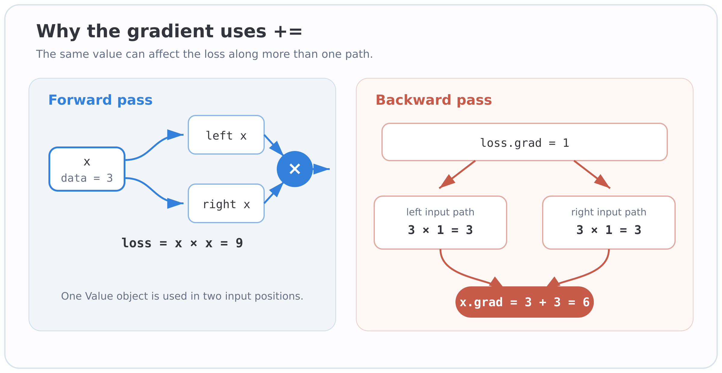
The part I struggled with was why the code adds to a gradient instead of replacing it. This example helped:

loss = x * x

x affects the result through both sides of the multiplication. If x is 3, each side contributes 3 to the gradient, and they have to be summed to get the expected derivative of 6. In a neural network, one weight can affect the loss through many paths, and its gradient is the sum of all of them. PyTorch does this with tensors and many more operations, but the process is the same.

After that, loss.backward() felt a lot less magical.

Putting the Transformer Together

With linear layers, softmax, and RMSNorm implemented, I could assemble the GPT. What surprised me was how little new machinery that needed. A linear layer is multiplication and addition. Softmax is exponentials, addition, and division. RMSNorm is squares, an average, and a square root. Autograd already supported all of those, so the full model just built one much bigger calculation graph.

At a high level, the model looked like this:

token and position embeddings
  -> attention
  -> MLP
  -> attention
  -> MLP
  -> scores for the next word

Normalization and residual connections wrap those pieces. Attention lets positions share information, and the MLP processes each position separately.

Residual connections made more sense once I stopped thinking of a layer as replacing the representation. The layer calculates an update that gets added to what was already there. If it has nothing useful to add yet, the original values still pass straight through, and gradients get the same shortcut going backward.

Attention Took the Longest

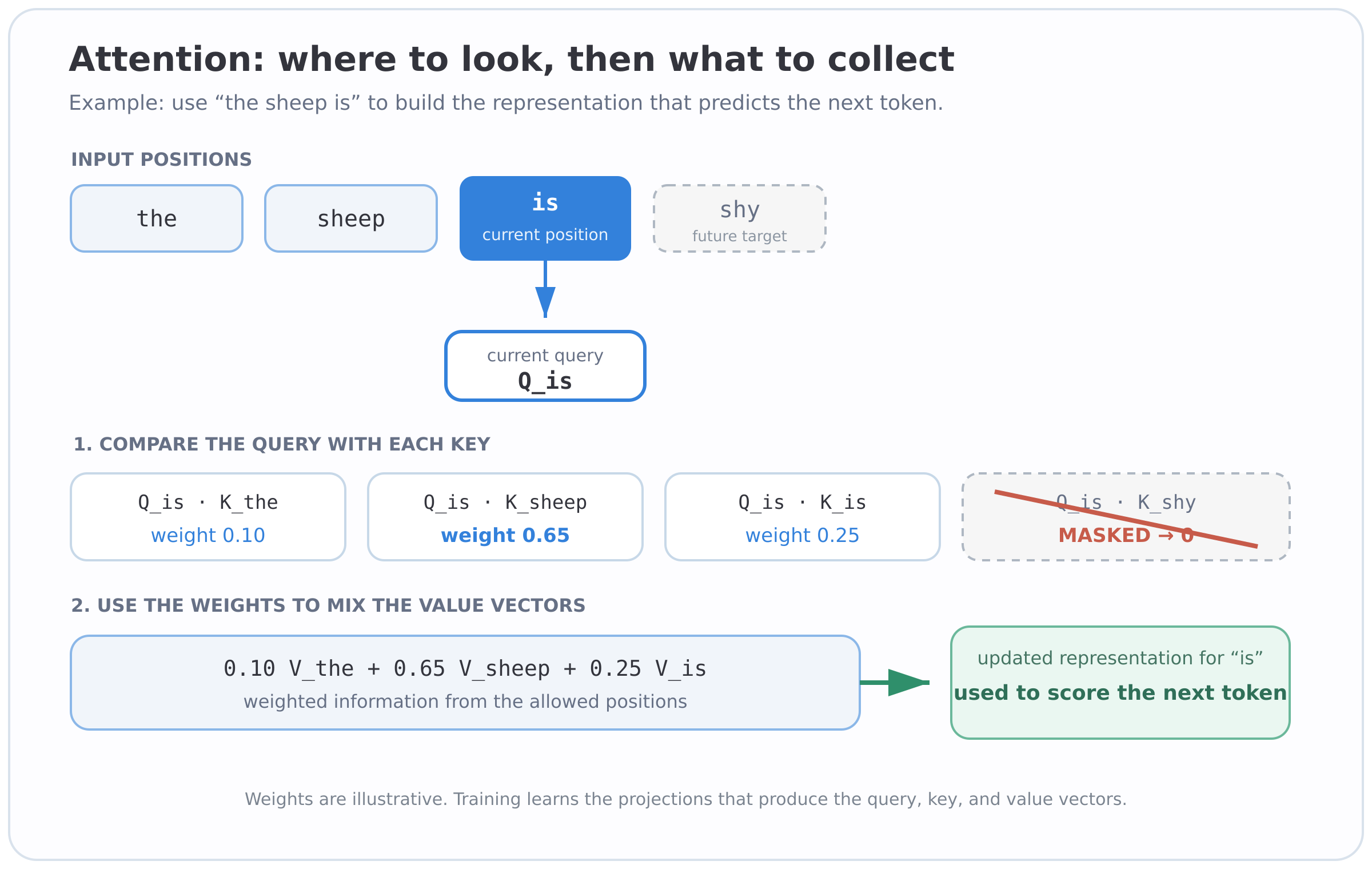
Attention was the main thing I wanted to understand going in, and the part I went back over the most. I’d seen queries, keys, and values explained many times but still couldn’t picture the calculation. What helped was splitting it into two steps: queries and keys decide how much each position should attend to each other position, then those weights decide how much of each value vector to bring back. Queries and keys answer “where should I look?”, and values are what gets collected.

These vectors are recalculated from each token’s current representation, so the model isn’t learning a fixed rule that bank always attends to river. It learns the matrices that produce useful matches given the surrounding text.

The causal mask was simpler: a position can look at itself and anything before it, but not later words, or it could see the answer during training.

The scalar attention code made the order of operations easy to follow:

query = linear(hidden, attention.query)
key = linear(hidden, attention.key)
value = linear(hidden, attention.value)

cache_keys.append(key)
cache_values.append(value)

scores = [
    dot(head_query, head_key) / sqrt(head_dim)
    for head_key in head_keys
]
weights = softmax(scores)
attended = weighted_sum(weights, head_values)

The real implementation spells out dot and weighted_sum with scalar Value operations, but this is the shape of it: make three projections, compare the query with stored keys, turn scores into weights, and combine the values.

Multi-head attention took a bit longer, because I pictured each head as more independent than it is. The 32 numbers representing a token are split across four heads of eight. Each head runs attention on its slice, and the results are joined and mixed by another linear layer. I didn’t come away with an intuition for what each head learns, which is probably the wrong thing to expect from such a small model, but I did understand how the calculation is divided up and put back together.

Getting the First Model to Learn Anything

I trained the scalar model on 20 simple sentences. It had 1,744 parameters, one attention head, one layer, and a context of eight words. An untrained model choosing between 57 tokens should start at a loss of about 4.04, and after 100 steps it was down to 2.36.

Some generated sentences were surprisingly reasonable:

the seed is shy
the brave bell is scared
the gray house

Others looked more like what I expected:

the am drums is the seed
the egg child dog i

Both kinds showed more than the loss did. The model had picked up patterns like the ... is ... without enough data or capacity to use them consistently.

I originally planned to reproduce the book’s much larger scalar training run. Once I saw how slowly all those Value objects ran in Python, I reconsidered. The small run already showed that loss went down, the saved model reloaded, and it generated valid words, which was enough to show everything was connected. The slowness was also a pretty good introduction to why tensor libraries exist.

Training and Generating Are Almost the Same Loop

In both training and generation, the model predicts what comes next. During training, the real next word is known, the loss measures how far off the prediction was, and the weights update. During generation, the code picks one of the predicted words, appends it, and runs the model again.

That made temperature, top-k, and top-p feel less mysterious. They don’t change what the model knows, only how the next word is picked from its scores.

Fine-tuning was similar. I expected a different process, but it was mostly the same loop with a saved model, a smaller dataset, and gentler updates. The tricky parts were keeping the original tokenizer and not overwriting too much of what the model had already learned.

Rebuilding It in PyTorch

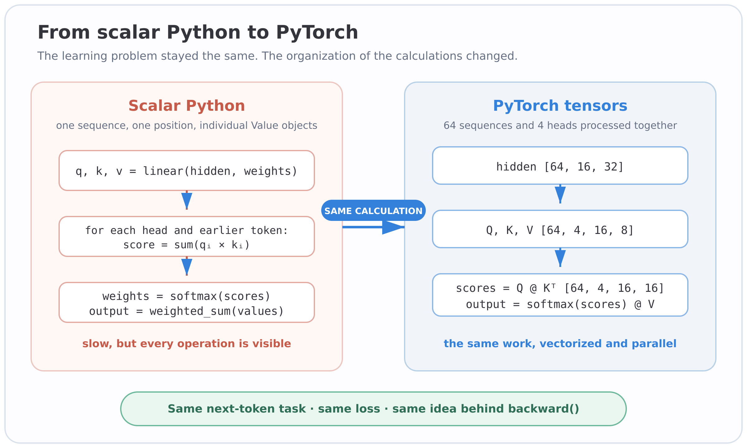
Moving to PyTorch is where the scalar work paid off. It didn’t feel like a different implementation. I could recognize the same operations, just applied to many values at once.

The new struggle was tensor shapes. The PyTorch model trained on 64 sequences of 16 positions, each with 32 features split into four heads:

hidden values:    [64, 16, 32]
attention heads:  [64, 4, 16, 8]
attention scores: [64, 4, 16, 16]

Focusing on the last [16, 16] helped: for each of the 16 positions, a score for every position it could attend to. The other two dimensions are PyTorch doing that for all 64 sequences and four heads at once.

Most of the attention calculation became a few tensor operations:

query = self._split_heads(self.query(hidden), self.config.n_head)
key = self._split_heads(self.key(hidden), self.config.n_head)
value = self._split_heads(self.value(hidden), self.config.n_head)

scores = query @ key.transpose(-2, -1)
scores = scores / sqrt(self.config.head_dim)
allowed = self.causal_mask[:sequence_length, :sequence_length]
scores = scores.masked_fill(~allowed, float("-inf"))
weights = F.softmax(scores, dim=-1)
attended = weights @ value

It’s the same sequence as the scalar version: one matrix multiplication does all the query-key comparisons, and another combines the values.

Batching had looked like extra complexity in PyTorch language-model code, but the learning problem doesn’t change. A batch just packs many next-token examples into one tensor operation so they run efficiently.

Each training step handled 64 windows of 16 tokens, or 1,024 next-token predictions at once. Over 5,000 steps the loss went like this:

step     0 | train 6.46 | validation 6.45
step  2500 | train 2.29 | validation 2.44
step  4999 | train 2.19 | validation 2.44

The model generated the sheep is by the tent, about what I expected from a small set of simple sentences. More importantly, it trained fast enough to be the baseline for later experiments. I could also watch training loss keep improving after validation loss had stalled, which gave me something concrete to call overfitting rather than just a definition.

The training step ended up as the familiar PyTorch pattern:

inputs, targets = get_batch(...)
_, loss = model(inputs, targets)

optimizer.zero_grad()
loss.backward()
optimizer.step()

I could now connect each line to the scalar version: build the graph on the forward pass, clear old gradients, walk the graph backward, update the weights.

Where I Ended Up

I wouldn’t claim to understand every detail of transformers. I had to revisit plenty of things, especially tensor dimensions, normalization, and how attention heads are laid out in memory.

But I could follow a token through the model: its ID picks an embedding, attention mixes in information from earlier positions, the model scores every possible next word, that becomes one loss, and the gradient finds its way back to the weights. PyTorch no longer felt like a black box. loss.backward() was a bigger version of the graph traversal I had written, and batching was many copies of the same prediction task.

The final model wasn’t interesting for what it generated. It was interesting because I understood enough of it to start changing things and have some idea what those changes meant. That’s what I did next: varying the model’s size and architecture one part at a time to see what actually happened.