Note that this is taken from Chapter 3 of the Hand-on Machine Learning book.
It is recommended you review my Classifying the MNIST dataset - The Hello, World of ML article to get a background on the MNIST dataset
import matplotlib as mpl
import matplotlib.pyplot as plt
import numpy as np
import pandas as pd
import sklearn

sklearn.__version__'1.1.1'Get the dataset
from sklearn.datasets import fetch_openml
mnist = fetch_openml("mnist_784", version=1)
mnist['data'].to_csv('./mnist_data.csv')
mnist['target'].to_csv('./mnist_target.csv')
mnist.keys()

# mnist = dict()
# mnist['data'] = pd.read_csv('./mnist_data.csv', index_col=0)
# mnist['target'] = pd.read_csv('./mnist_target.csv', index_col=0).squeeze('columns')
dict_keys(['data', 'target', 'frame', 'categories', 'feature_names', 'target_names', 'DESCR', 'details', 'url'])Convert the target to a number, and split the dataset into a train and test set
X, y = mnist["data"].to_numpy(), mnist["target"].to_numpy()
y = y.astype(np.uint8)

X_train, X_test, y_train, y_test = X[:60000], X[60000:], y[:60000], y[60000:]
The Task - 97% Accuracy Classifier
Try to build a classifier for the MNIST dataset that achieves over
97% accuracy on the test set. Hint: the
KNeighborsClassifier works quite well for this task; you
just need to find good hyperparameter values (try a grid search on the
weights and n_neighbors hyperparameters).
Let’s build a KNeighborsClassifier model using
GridSearchCV to find the best parameters.
NOTE that this cell make take 16+ hours to run
from sklearn.neighbors import KNeighborsClassifier
from sklearn.model_selection import GridSearchCV

param_grid = [{'weights': ["uniform", "distance"], 'n_neighbors': [3, 4, 5]}]

knn_clf = KNeighborsClassifier()
grid_search = GridSearchCV(knn_clf, param_grid, cv=5, verbose=3)
grid_search.fit(X_train, y_train)
What were our best parameters?
grid_search.best_params_{'n_neighbors': 4, 'weights': 'distance'}What was our best score?
grid_search.best_score_0.9716166666666666Looks promising. Now lets run the best model on the test set
from sklearn.metrics import accuracy_score

y_pred = grid_search.predict(X_test)
accuracy_score(y_test, y_pred)0.9714Looks like we achieved 97%!
The Task - Data Augmentation
Write a function that can shift the MNIST image in any direction (left, right, up, or down) by one pixel. Then, for each image in the training set, create four shifted copies (one per direction) and add them to the training set. Finally, train your best model on this expanded training set and measure its accuracy on the test set. You should observe that your model performs even better now. This technique of artifically growing the training set is called data augmentation or training set expansion.
We can use scipy’s shift function the shift the
image
from scipy.ndimage import shift

def shift_image(image, dx, dy):
    image = image.reshape((28, 28))
    shifted_image = shift(image, [dy, dx], cval=0, mode="constant")
    return shifted_image.reshape([-1])
Let’s run a quick example by shifting a single image 5 pixels down and 5 pixels left.
image = X_train[1000]
shifted_image_down = shift_image(image, 0, 5)
shifted_image_left = shift_image(image, -5, 0)

plt.figure(figsize=(12,3))
plt.subplot(131)
plt.title("Original", fontsize=14)
plt.imshow(image.reshape(28, 28), interpolation="nearest", cmap="Greys")
plt.subplot(132)
plt.title("Shifted down", fontsize=14)
plt.imshow(shifted_image_down.reshape(28, 28), interpolation="nearest", cmap="Greys")
plt.subplot(133)
plt.title("Shifted left", fontsize=14)
plt.imshow(shifted_image_left.reshape(28, 28), interpolation="nearest", cmap="Greys")
plt.show()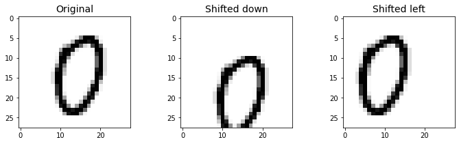
Those look good. Lets create the augmented dataset by adding an image shifted up, left, down and right.
X_train_augmented = [image for image in X_train]
y_train_augmented = [label for label in y_train]

for dx, dy in ((1, 0), (-1, 0), (0, 1), (0, -1)):
    for image, label in zip(X_train, y_train):
        X_train_augmented.append(shift_image(image, dx, dy))
        y_train_augmented.append(label)

X_train_augmented = np.array(X_train_augmented)
y_train_augmented = np.array(y_train_augmented)
We should make sure we shuffle the dataset to make sure the images that were generated from the original are not all next to each other
shuffle_idx = np.random.permutation(len(X_train_augmented))
X_train_augmented = X_train_augmented[shuffle_idx]
y_train_augmented = y_train_augmented[shuffle_idx]
Now let’s create a new KNeighborsClassifier and train it
with the augmented data:
knn_clf = KNeighborsClassifier(**grid_search.best_params_)
knn_clf.fit(X_train_augmented, y_train_augmented)
KNeighborsClassifier(n_neighbors=4, weights='distance')In a Jupyter environment, please rerun this cell to show the HTML representation or trust the notebook.
On GitHub, the HTML representation is unable to render, please try loading this page with nbviewer.org.
KNeighborsClassifier(n_neighbors=4, weights='distance')
Finally, let’s test our classifier trained with the augmented data on the test set to see what our accuracy score is.
NOTE that this cell may take up to an hour to run
y_pred = knn_clf.predict(X_test)
accuracy_score(y_test, y_pred)0.9763By simply augmenting the data, we got roughly a 0.5% accuracy boost!