Principal Component Analysis (PCA) is by far the most popular dimensionality reduction algorithm. First it identifies the hyperplace that lies closest to the data, and then it projects the data onto it.
Preserving the Variance
Before you can project the training set onto a lower-dimensional hyperplace, you first need to choose the right hyperplace. For example, in the image below, a simple 2D dataset is represented on the left plot, along with three different axes (i.e., 1D hyperplanes). On the right is the result of the projection of the dataset onto each of these axes. It can be seen that the projection onto the solid line preserves the maximum variance, while the projection onto the dotted line preserves very little variance and the projection onto the dashed line preserves an intermediate amount of variance.
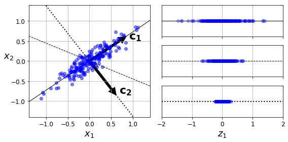
It seems reasonable to select the axis that preserves the maximum amount of variance, as it will most likely lose less information than the other projections. Another way to justify this choice is that it is the axis that minimizes the mean squared distance between the original dataset and its projection onto that axis. This is the rather simple idea behind PCA.
Principal Components
PCA identifies the axis that accounts for the largest amount of variance in the training set. In the image above, it is the solid line. It also finds a second axis, orthogonal to the first one, that accounts for the largest amount of the remaining variance. In this 2D example there is no choice: it is the dotted line. If it were a higher-dimensional dataset, PCA would also find a third axis, orthogonal to both previous axes, and a fourth, and a fifth, and so on - as many axes as the number of dimensions in the dataset.
The ith axis is called the ith principal component (PC) of the data. In the example above, the first PC is the axis on which vector c1 lies, and the second PC is the axis on which vector c2 lies.
So how can you find the principal components of a training set? Luckily, there is a standard matrix factorization technique called Singular Value Decomposition (SVD) that can decompose the training set matrix X into the matrix multiplication of three matrices U Σ VT, where V contains the unit vectors that define all principal components that we are looking for:
V = [c1 c2 … cn]
Projecting Down to d Dimensions
Once you have identified all the principal components, you can reduce the dimensionality of the dataset down to d dimensions by projecting it onto the hyperplace defined by the first d principal components. Selecting this hyperplane ensures that the projection will preserve as much variance as possible.
To project the training set onto the hyperplace and obtain a reduced dataset Xd-proj of dimensionality d, compute the matrix multiplication of the training set matrix X by the matrix Wd, defined as the matrix containing the first d columns of V:
Xd-proj = XWd
Using Scikit-Learn
Scikit-Learn’s PCA class uses SVD decomposition to implement PCA. The following code applies PCA to reduce the dimensionality of the dataset downt o two dimensions (note that it automatically takes care of centering the data):
from sklearn.decomposition import PCA

pca = PCA(n_components=2)
X2D = pca.fit_transform(x)
After fitting the PCA transformer to the dataset, its
components attribute holds the transpose of
Wd (e.g., the unit vectore that defines the
first principal component is equal to pca.components.T[:,
0]).
Explained Variance Ratio
Another useful piece of information is the explained variance
ratio of each principal component, available via the
explainedvariance_ratio variable. The ratio
indicates the proportion of the dataset’s variance that lies along each
principal component. For example:
>>> pca.explained_variance_ratio_
array([0.84248607, 0.14631839])
This output tells you that 84.2% of the dataset’s variance lies along the first PC, and 14.6% lies along the second PC. This leaves less than 1.2% for the third PC, so it is reasonable to assume that the third PC probably carries little information.
Choosing the Right Number of Dimensions.
Instead of arbitrarily choosing the number of dimensions to reduce down to, it is simpler to choose the number of dimensions that add up to a sufficiently large portion of the variance (e.g., 95%). Unless, of course, you are reducing dimensionality for data visualization - in that case you will want to reduce the dimensionality down to 2 or 3.
The following code performs PCA without reducing dimensionality, then computes the minimum number of dimensions required to preserve 95% of the traiing set’s variance:
pca = PCA()
pca.fit(X_train)
cumsum = np.cumsum(pca.explained_variance_ratio_)
d = np.argmax(cumsum >= 0.95) + 1
You could then set n_components=d and run PCA again, But
there is a much better option: instead of specifying the number of
principal components you want to preserve, you can set
n_components to be a float between 0.0. and 1.0, indicating
the ratio of variance you wish to preserve:
pca = PCA(n_components=0.95)
X_reduced = pca.fit_transform(X_train)
Yet another option is to plot the explained variance as a function of
the number of dimensions (simply plot cumsum). There will
usually be an elbow in the curve, where the explained variance stops
growing fast.